Spatial Enrichment Analysis

Spatial transcriptomics technologies yield many molecular readouts that are hard to interpret by themselves. One way of summarizing this information is by inferring enrichment scores from prior knowledge.

In this notebook, we demonstrate how to use decoupler to infer transcription factor (TF) and pathway enrichment scores from a spatial transcriptomics (Visium) human dataset.

The dataset includes 4k mini-bulk spots from a chronic active multiple sclerosis lesion [LMBiMRF+24]. It publicly available at GEO (GSE279183).

Loading Packages

import warnings

import scanpy as sc
import decoupler as dc

warnings.filterwarnings("ignore", category=FutureWarning)
sc.set_figure_params(figsize=(3, 3), frameon=False)

Loading The Dataset

adata = dc.ds.msvisium()
adata

AnnData object with n_obs × n_vars = 3839 × 14940
    obs: 'array_row', 'array_col', 'niches'
    uns: 'spatial'
    obsm: 'spatial'

The obtained anndata.AnnData consist of raw integer transcript counts for ~4k mini-bulk measurements for ~15k genes.

The following step normalizes the data and stores it into a layer for later use.

sc.pp.normalize_total(adata, target_sum=1e4)
sc.pp.log1p(adata)

adata.layers["norm"] = adata.X.copy()

The cell metadata stored in anndata.AnnData.obs can be inspected.

adata.obs

	array_row	array_col	niches
AAACAAGTATCTCCCA-1	50	102	LC
AAACACCAATAACTGC-1	59	19	PPWM
AAACAGAGCGACTCCT-1	14	94	VI
AAACAGCTTTCAGAAG-1	43	9	PPWM
AAACAGGGTCTATATT-1	47	13	PPWM
...	...	...	...
TTGTTGTGTGTCAAGA-1	31	77	LC
TTGTTTCACATCCAGG-1	58	42	LR
TTGTTTCATTAGTCTA-1	60	30	PPWM
TTGTTTCCATACAACT-1	45	27	PPWM
TTGTTTGTGTAAATTC-1	7	51	LC

3839 rows × 3 columns

The dataset also includes tissue annotations from the original publication:

• GM: Grey Matter

• LC: Lesion Core

• LR: Lesion Rim

• PPWM: PeriPlaque White Matter

• VI: Vascular Infiltrating

The H&E image and the different annotated regions (niches) can be visualized.

sc.pl.spatial(adata, color=[None, "niches"], size=1.5, ncols=1)

Spatial Weighting

Spatial data are often sparse. To address this, spatial information can be leveraged to impute gene expression based on the expression levels of nearby spatial neighbors [DSchaferF+24].

This is achieved by generating spatial weights for each spot and applying them to the gene expression values, effectively smoothing the data.

dc.pp.knn(adata, key="spatial", bw=100, cutoff=0.1)

The spatial weights assigned to each spot can then be visualized.

# Plot the spatial weights of one spot
adata.obs["conn"] = adata.obsp["spatial_connectivities"][0].toarray().ravel()
sc.pl.spatial(adata, color="conn", size=1.5)

It can be observed that for a given spot, the spatial weight is maximal at the spot itself and decreases with increasing distance to other spots.

Adjust the bandwith (bw) to increase or decrease the radius to consider.

The gene expression values can now be spatially weighted.

# Update X with spatially weighted gene exression
adata.X = adata.obsp["spatial_connectivities"].dot(adata.X)

The original log-normalized counts can be plotted alongside the newly spatially transformed values.

genes = ["MOG", "CD163", "IGKC"]

# Log-normalized counts
sc.pl.spatial(adata, color=genes, size=1.5, layer="norm")

# Spatially weighted gene expression
sc.pl.spatial(adata, color=genes, size=1.5)

After smoothing, spots surrounded by other spots expressing the same gene will have higher values compared to spots lacking neighboring spots with high values, even if those spots themselves had high values of expression.

Gene expression for these genes appears to exhibit spatial compartmentalization.

Enrichment analysis

Enrichment analysis tests whether a specific set of omics features is “overrepresented” or “coordinated” in the measured data compared to a background distribution. These sets are predefined based on existing biological knowledge and may vary depending on the omics technology used.

Enrichment analysis requires the use of an enrichment method, and several options are available. In the original manuscript of decoupler [BiMVSB+22], we benchmarked multiple methods and found that the univariate linear model (ulm) outperformed the others. Therefore, we will use ulm in this vignette.

The scores from decoupler.mt.ulm() should be interpreted such that larger magnitudes indicate greater significance, while the sign reflects whether the features in the set are overrepresented (positive) or underrepresented (negative) compared to the background.

Transcription factor scoring from gene regulatory networks

Transcription factors (TFs) are genes that, once translated into proteins, bind to DNA and regulate the expression of other genes by either promoting or inhibiting their transcription. Gene Regulatory Networks (GRNs) capture these TF-gene interactions and can be constructed from prior knowledge or inferred from omics data. The fundamental unit of a GRN is a TF and its associated target genes, collectively known as a regulon. Each regulon functions as a gene set in enrichment analysis.

Although TFs are measured in transcriptomic data, their transcript levels often do not reflect their actual activity in a given cell. Instead, scoring TFs through enrichment analysis based on the expression of their target genes provides a more accurate representation of their regulatory activity [BiMWMullerD+23].

CollecTRI network

CollecTRI is a comprehensive resource containing a curated collection of TFs and their transcriptional targets compiled from 12 different resources [MullerDTV+23]. This collection provides an increased coverage of transcription factors and a superior performance in identifying perturbed TFs compared to other literature based GRNs such as DoRothEA [GAHI+19]. Similar to DoRothEA, interactions are weighted by their mode of regulation (activation or inhibition).

In this tutorial we will use the human version but other organisms are available. We can use decoupler to retrieve it from the OmniPath server [TureiKSR16].

Note In this tutorial we use the network CollecTRI, but we could use any other GRN coming from an inference method such as CellOracle, pySCENIC or SCENIC+.

collectri = dc.op.collectri(organism="human")
collectri

	source	target	weight	resources	references	sign_decision
0	MYC	TERT	1.0	DoRothEA-A;ExTRI;HTRI;NTNU.Curated;Pavlidis202...	10022128;10491298;10606235;10637317;10723141;1...	PMID
1	SPI1	BGLAP	1.0	ExTRI	10022617	default activation
2	SMAD3	JUN	1.0	ExTRI;NTNU.Curated;TFactS;TRRUST	10022869;12374795	PMID
3	SMAD4	JUN	1.0	ExTRI;NTNU.Curated;TFactS;TRRUST	10022869;12374795	PMID
4	STAT5A	IL2	1.0	ExTRI	10022878;11435608;17182565;17911616;22854263;2...	default activation
...	...	...	...	...	...	...
42985	NFKB	hsa-miR-143-3p	1.0	ExTRI	19472311	default activation
42986	AP1	hsa-miR-206	1.0	ExTRI;GEREDB;NTNU.Curated	19721712	PMID
42987	NFKB	hsa-miR-21	1.0	ExTRI	20813833;22387281	default activation
42988	NFKB	hsa-miR-224-5p	1.0	ExTRI	23474441;23988648	default activation
42989	AP1	hsa-miR-144-3p	1.0	ExTRI	23546882	default activation

42990 rows × 6 columns

Scoring

TF scores can be easily computed by running the ulm method.

dc.mt.ulm(data=adata, net=collectri)

Scores can be then extracted as a new anndata.AnnData object.

score = dc.pp.get_obsm(adata=adata, key="score_ulm")
score

AnnData object with n_obs × n_vars = 3839 × 660
    obs: 'array_row', 'array_col', 'niches', 'conn'
    uns: 'spatial', 'log1p', 'niches_colors'
    obsm: 'spatial', 'score_ulm', 'padj_ulm'

The obtained scores can be visualized.

tf = "RFX5"
sc.pl.spatial(score, color=[tf, "niches"], cmap="RdBu_r", vcenter=0, size=1.5, title=[f"{tf} score", "niches"])
sc.pl.violin(score, keys=tf, groupby="niches", rotation=90, ylabel=f"{tf} score")

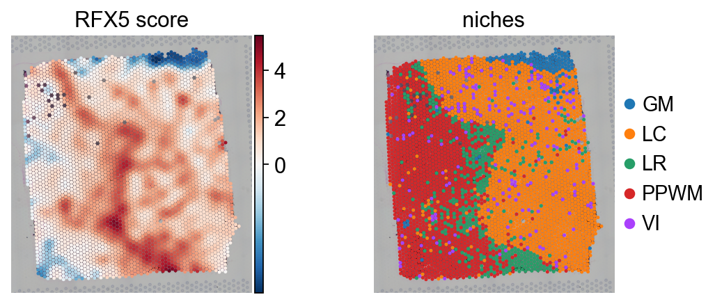
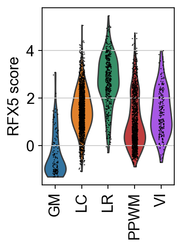
Here, the TF RFX5, a key regulator for antigen-presenting cells, exhibits a strong spatial pattern, showing greater activity in the lesion rim (LR) compared to other areas of the tissue. This aligns with the known fact that these cells are present in this region to engulf cellular debris coming from the lesion core.

This can be compared with the actual expression values of the RFX5 gene.

tf = "RFX5"
sc.pl.spatial(adata, color=[tf, "niches"], size=1.5, title=[f"{tf} expression", "niches"])
sc.pl.violin(adata, keys=tf, groupby="niches", rotation=90, ylabel=f"{tf} expression")

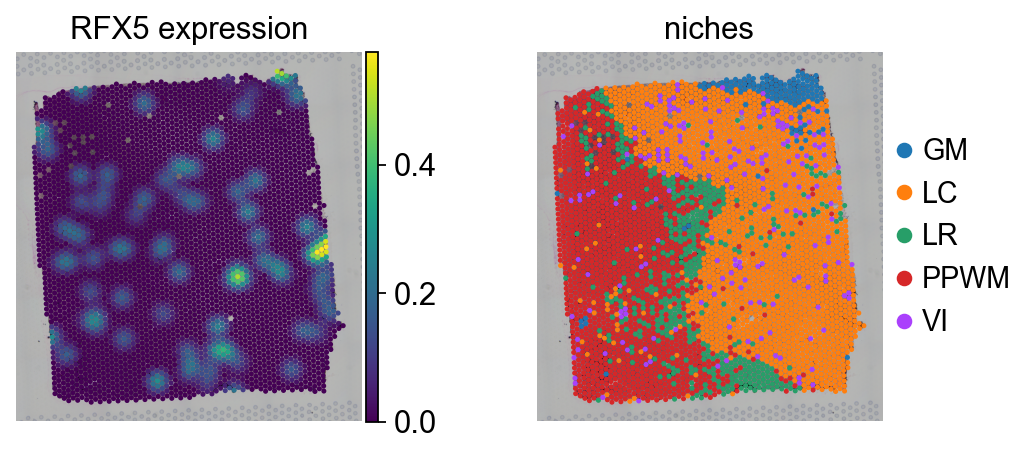
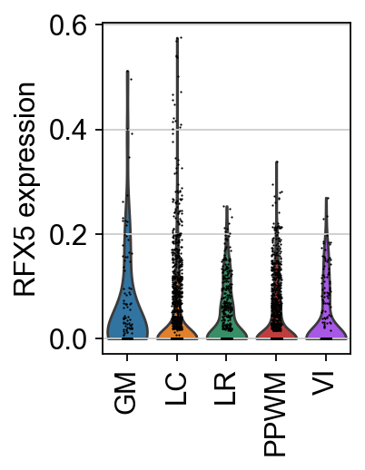
When we look at the expression of the TF RFX5 there is no spatial pattern, as it is randomly expressed across the tissue.

TF expression tends to be sporadic and insufficiently informative to determine whether a TF is active in a cell, underscoring the importance of using enrichment scores for interpreting biological data [BiMWMullerD+23].

Next, marker TFs for each niche can be identified.

df = dc.tl.rankby_group(adata=score, groupby="niches", reference="rest", method="t-test_overestim_var")
df = df[df["stat"] > 0.0]
df

	group	reference	name	stat	meanchange	pval	padj
0	LC	rest	SOX2	67.507158	1.769902	0.000000	0.000000
1	LC	rest	LHX2	65.869208	1.727253	0.000000	0.000000
2	LC	rest	POU3F1	58.382363	2.273192	0.000000	0.000000
3	LC	rest	SNAI1	57.754488	1.321344	0.000000	0.000000
4	LC	rest	NFIC	57.671362	1.370289	0.000000	0.000000
...	...	...	...	...	...	...	...
3289	GM	rest	ARID1A	0.272784	0.012372	0.785291	0.797372
3290	GM	rest	NFE2L2	0.259121	0.022869	0.795821	0.806823
3294	GM	rest	FOXD1	0.168305	0.012613	0.866477	0.873091
3297	GM	rest	KMT2B	0.070595	0.002892	0.943776	0.946644
3299	GM	rest	LHX8	0.016945	0.000832	0.986494	0.986494

1611 rows × 7 columns

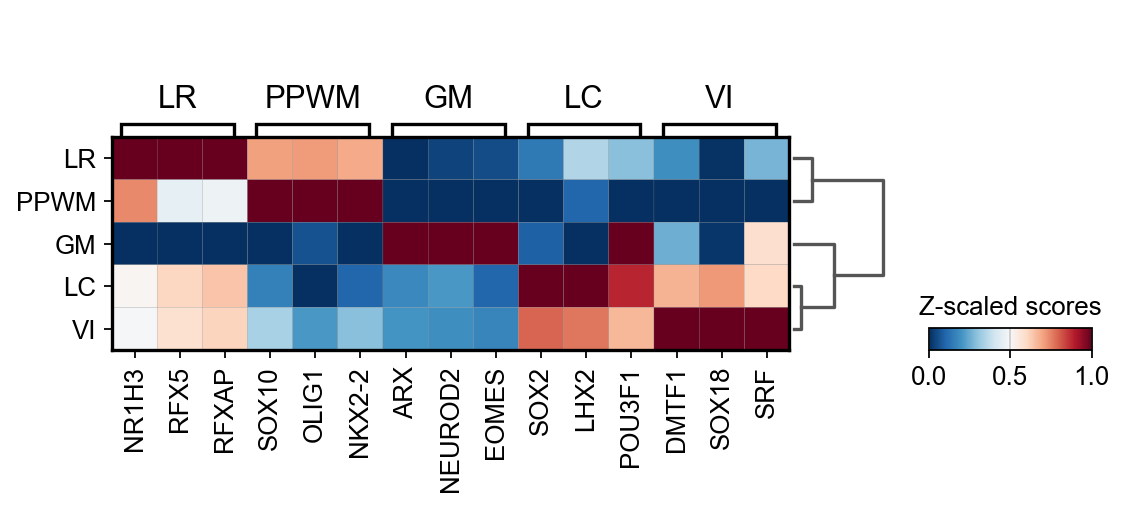
The top 3 TF markers per niche can then be extracted.

n_markers = 3
source_markers = (
    df.groupby("group")
    .head(n_markers)
    .drop_duplicates("name")
    .groupby("group")["name"]
    .apply(lambda x: list(x))
    .to_dict()
)
source_markers

{'GM': ['ARX', 'NEUROD2', 'EOMES'],
 'LC': ['SOX2', 'LHX2', 'POU3F1'],
 'LR': ['NR1H3', 'RFX5', 'RFXAP'],
 'PPWM': ['SOX10', 'OLIG1', 'NKX2-2'],
 'VI': ['DMTF1', 'SOX18', 'SRF']}

The obtained markers can be plotted

sc.pl.matrixplot(
    adata=score,
    var_names=source_markers,
    groupby="niches",
    dendrogram=True,
    standard_scale="var",
    colorbar_title="Z-scaled scores",
    cmap="RdBu_r",
)

WARNING: dendrogram data not found (using key=dendrogram_niches). Running `sc.tl.dendrogram` with default parameters. For fine tuning it is recommended to run `sc.tl.dendrogram` independently.

Individual TFs can be examined by plotting their score distributions.

tf = "OLIG1"
sc.pl.spatial(score, color=[tf, "niches"], cmap="RdBu_r", vcenter=0, size=1.5, title=[f"{tf} score", "niches"])
sc.pl.violin(score, keys=[tf], groupby="niches", rotation=90, ylabel=f"{tf} score")

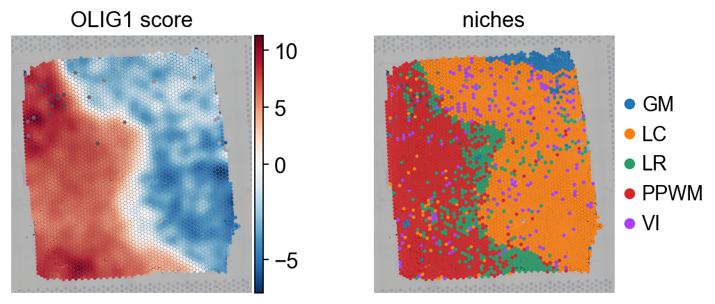
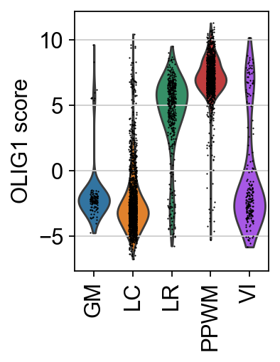
Here, the TF activities for OLIG1 can be observed. OLIG1 is a known marker TF for oligodendrocytes, which are present in the PPWM.

Pathway Scoring

The same approach used for TF scoring can also be applied to pathways. Numerous databases provide curated pathway gene sets, with one of the most well-known being MSigDB, which includes several collections [LSP+11]. These and many other resources can be accessed using the function decoupler.op.resource(). To view the list of available databases, use decoupler.op.show_resources().

PROGENy Pathway Genes

PROGENy is a comprehensive resource that provides a curated collection of pathways and their target genes, along with weights for each interaction [SKK+18].

Below is a brief description of each pathway:

• Androgen: involved in the growth and development of the male reproductive organs

• EGFR: regulates growth, survival, migration, apoptosis, proliferation, and differentiation in mammalian cells

• Estrogen: promotes the growth and development of the female reproductive organs

• Hypoxia: promotes angiogenesis and metabolic reprogramming when O2 levels are low

• JAK-STAT: involved in immunity, cell division, cell death, and tumor formation

• MAPK: integrates external signals and promotes cell growth and proliferation

• NFkB: regulates immune response, cytokine production and cell survival

• p53: regulates cell cycle, apoptosis, DNA repair and tumor suppression

• PI3K: promotes growth and proliferation

• TGFb: involved in development, homeostasis, and repair of most tissues

• TNFa: mediates haematopoiesis, immune surveillance, tumour regression and protection from infection

• Trail: induces apoptosis

• VEGF: mediates angiogenesis, vascular permeability, and cell migration

• WNT: regulates organ morphogenesis during development and tissue repair

This is how to access to it.

progeny = dc.op.progeny(organism="human")
progeny

	source	target	weight	padj
0	Androgen	TMPRSS2	11.490631	2.384806e-47
1	Androgen	NKX3-1	10.622551	2.205102e-44
2	Androgen	MBOAT2	10.472733	4.632376e-44
3	Androgen	KLK2	10.176186	1.944410e-40
4	Androgen	SARG	11.386852	2.790210e-40
...	...	...	...	...
62456	p53	ENPP2	2.771405	4.993215e-02
62457	p53	ARRDC4	3.494328	4.996747e-02
62458	p53	MYO1B	-1.148057	4.997905e-02
62459	p53	CTSC	-1.784693	4.998864e-02
62460	p53	NAA50	-1.435013	4.998884e-02

62461 rows × 4 columns

Scoring

Pathway scores can be easily computed by running the ulm method.

dc.mt.ulm(data=adata, net=progeny)

Scores can be then extracted.

score = dc.pp.get_obsm(adata=adata, key="score_ulm")
score

AnnData object with n_obs × n_vars = 3839 × 14
    obs: 'array_row', 'array_col', 'niches', 'conn'
    uns: 'spatial', 'log1p', 'niches_colors', 'pca', 'dendrogram_niches'
    obsm: 'spatial', 'score_ulm', 'padj_ulm'

And visualized.

pw = "TNFa"
sc.pl.spatial(score, color=[pw, "niches"], cmap="RdBu_r", vcenter=0, size=1.5)
sc.pl.violin(score, keys=[pw], groupby="niches", rotation=90)

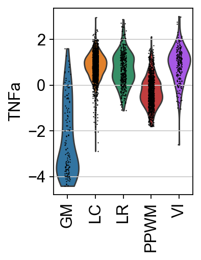
It seem that except in GM and PPWM, the pathway TNF-α, associated with inflamation, is more active.

Given that there are only 14 pathways, they can be directly visualized without the need for marker extraction.

sc.pl.matrixplot(
    adata=score,
    var_names=score.var_names,
    groupby="niches",
    dendrogram=True,
    standard_scale="var",
    colorbar_title="Z-scaled scores",
    cmap="RdBu_r",
)

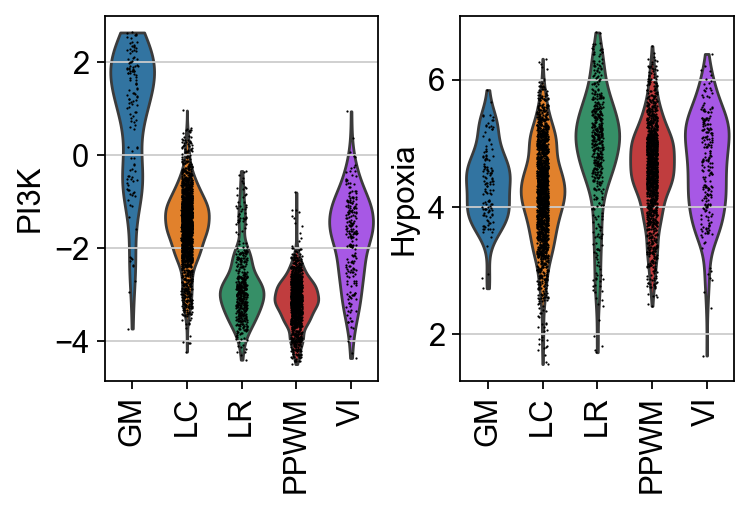
In this specific example, it can be observed that PI3K is more active in GM, while Hypoxia is more active in LR.

pws = ["PI3K", "Hypoxia"]
sc.pl.spatial(score, color=pws + ["niches"], cmap="RdBu_r", vcenter=0, size=1.5)
sc.pl.violin(score, keys=pws, groupby="niches", rotation=90)

Hallmark gene sets

Hallmark gene sets are curated collections of genes that represent specific, well-defined biological states or processes. They are part of MSigDB and were developed to reduce redundancy and improve interpretability compared to older, more overlapping gene set collections [LSP+11].

A total of 50 gene sets are provided, designed to be non-redundant, concise, and biologically coherent.

This is how to access them.

hallmark = dc.op.hallmark(organism="human")
hallmark

	source	target
0	IL2_STAT5_SIGNALING	MAFF
1	COAGULATION	MAFF
2	HYPOXIA	MAFF
3	TNFA_SIGNALING_VIA_NFKB	MAFF
4	COMPLEMENT	MAFF
...	...	...
7313	PANCREAS_BETA_CELLS	STXBP1
7314	PANCREAS_BETA_CELLS	ELP4
7315	PANCREAS_BETA_CELLS	GCG
7316	PANCREAS_BETA_CELLS	PCSK2
7317	PANCREAS_BETA_CELLS	PAX6

7318 rows × 2 columns

Scoring

Pathway scores can be easily computed by running the ulm method.

dc.mt.ulm(data=adata, net=hallmark)

Scores can be then extracted.

score = dc.pp.get_obsm(adata=adata, key="score_ulm")
score

AnnData object with n_obs × n_vars = 3839 × 50
    obs: 'array_row', 'array_col', 'niches', 'conn'
    uns: 'spatial', 'log1p', 'niches_colors', 'pca', 'dendrogram_niches'
    obsm: 'spatial', 'score_ulm', 'padj_ulm'

Next, marker gene sets for each niche can be identified.

df = dc.tl.rankby_group(adata=score, groupby="niches", reference="rest", method="t-test_overestim_var")
df = df[df["stat"] > 0]
df

	group	reference	name	stat	meanchange	pval	padj
0	LC	rest	UV_RESPONSE_DN	43.795912	1.108682	0.000000e+00	0.000000e+00
7	LC	rest	EPITHELIAL_MESENCHYMAL_TRANSITION	37.059294	1.122682	1.481980e-254	9.262372e-254
9	LC	rest	INTERFERON_GAMMA_RESPONSE	35.737296	1.155296	5.324817e-230	2.662408e-229
10	LC	rest	TNFA_SIGNALING_VIA_NFKB	31.496445	0.661386	1.507690e-191	6.853138e-191
11	LC	rest	ESTROGEN_RESPONSE_EARLY	30.861858	0.660593	2.228121e-183	9.283838e-183
...	...	...	...	...	...	...	...
234	GM	rest	ADIPOGENESIS	5.733774	0.747548	2.948604e-08	4.212292e-08
236	GM	rest	FATTY_ACID_METABOLISM	5.011884	0.467963	1.070111e-06	1.446096e-06
242	GM	rest	HEME_METABOLISM	3.116015	0.232688	2.048749e-03	2.382266e-03
243	GM	rest	ESTROGEN_RESPONSE_EARLY	2.888789	0.200897	4.349467e-03	4.942576e-03
245	GM	rest	DNA_REPAIR	1.536304	0.091333	1.258012e-01	1.367405e-01

128 rows × 7 columns

The top 3 set markers per cell type can then be extracted.

n_markers = 3
source_markers = (
    df.groupby("group")
    .head(n_markers)
    .drop_duplicates("name")
    .groupby("group")["name"]
    .apply(lambda x: list(x))
    .to_dict()
)
source_markers

{'GM': ['HEDGEHOG_SIGNALING',
  'PANCREAS_BETA_CELLS',
  'OXIDATIVE_PHOSPHORYLATION'],
 'LC': ['UV_RESPONSE_DN',
  'EPITHELIAL_MESENCHYMAL_TRANSITION',
  'INTERFERON_GAMMA_RESPONSE'],
 'LR': ['COAGULATION', 'COMPLEMENT', 'ALLOGRAFT_REJECTION'],
 'PPWM': ['SPERMATOGENESIS', 'BILE_ACID_METABOLISM', 'ANDROGEN_RESPONSE'],
 'VI': ['TNFA_SIGNALING_VIA_NFKB']}

And plotted.

sc.pl.matrixplot(
    adata=score,
    var_names=source_markers,
    groupby="niches",
    dendrogram=True,
    standard_scale="var",
    colorbar_title="Z-scaled scores",
    cmap="RdBu_r",
    swap_axes=True,
)

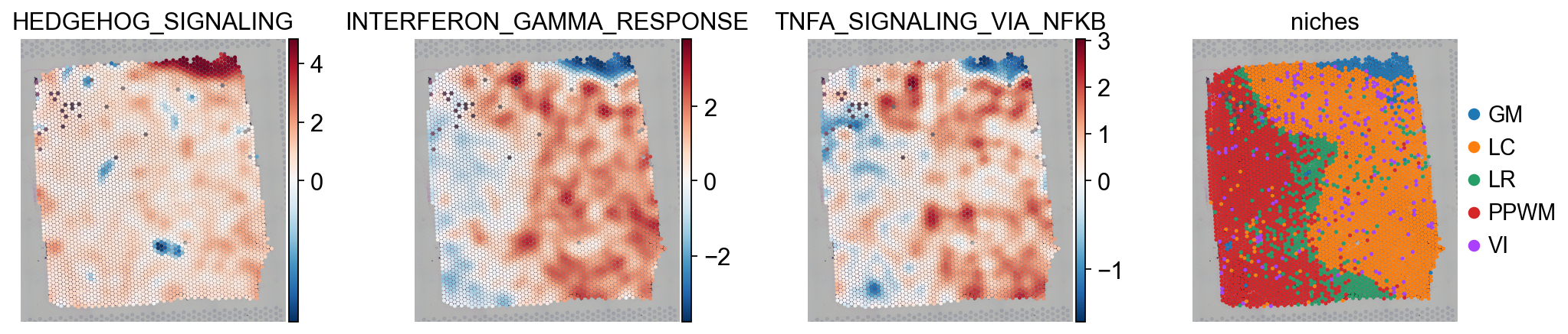
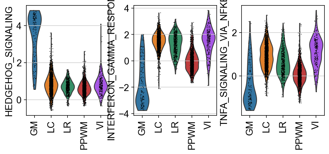
In this specific example, it can be observed that HEDGEHOG_SIGNALING is more active in GM, while INTERFERON_GAMMA_RESPONSE and TNFA_SIGNALING_VIA_NFKB are more active in LC and VI.

hms = ["HEDGEHOG_SIGNALING", "INTERFERON_GAMMA_RESPONSE", "TNFA_SIGNALING_VIA_NFKB"]
sc.pl.spatial(score, color=hms + ["niches"], cmap="RdBu_r", vcenter=0, size=1.5)
sc.pl.violin(score, keys=hms, groupby="niches", rotation=90)

References

{bibliography}