Pseudotime Enrichment Analysis

Analyzing omics data is not always as straightforward as comparing observations between two discrete groups, such as treatment against control. In some cases, the biological context exhibits a continuous nature, such as cell differentiation, disease progression, or developmental stages. In these scenarios, it is important to assess how features change along the continuous process and how enrichment scores that summarize these features vary across this axis.

This notebook demonstrates the use of decoupler to infer transcription factor (TF) and pathway enrichment scores from a mouse scRNA-seq dataset.

The dataset includes 1k donwsampled cells from the erytroid lineage during mouse gastrulation [PSGG+19], a continuous process that can be characterized by the inferrence of pseudotime.

Loading Packages

import numpy as np

import scanpy as sc
import decoupler as dc

sc.set_figure_params(figsize=(3, 3), frameon=False)

Loading The Dataset

adata = dc.ds.erygast1k()
adata

AnnData object with n_obs × n_vars = 801 × 8124
    obs: 'sample', 'stage', 'sequencing.batch', 'theiler', 'celltype'
    uns: 'celltype_colors', 'log1p'
    obsm: 'X_pca', 'X_umap'

The obtained anndata.AnnData consist of log-normalized transcript counts for ~1k cells with measurements for ~8k genes.

The cell metadata stored in anndata.AnnData.obs can be inspected.

adata.obs

	sample	stage	sequencing.batch	theiler	celltype
GTGGATTGCGTCTC	29	E8.5	3	TS12	Erythroid1
ACTGCCTGAACGGG	12	E7.75	2	TS11	Blood progenitors 2
TCCACTCTCTTCGC	36	E8.5	3	TS12	Erythroid3
GCAGCCGAGTGTTG	20	E7.5	2	TS11	Blood progenitors 2
GATCCCTGATCGTG	37	E8.5	3	TS12	Erythroid3
...	...	...	...	...	...
GACATTCTGGAACG	13	E7.75	2	TS11	Blood progenitors 2
ACAAATTGCGTGTA	36	E8.5	3	TS12	Erythroid3
TGCACGCTAACGTC	37	E8.5	3	TS12	Erythroid3
GCAGTTGAGGTTAC	16	E8.0	2	TS12	Erythroid1
ACGGTCCTTTTCAC	28	E8.25	2	TS12	Erythroid2

801 rows × 5 columns

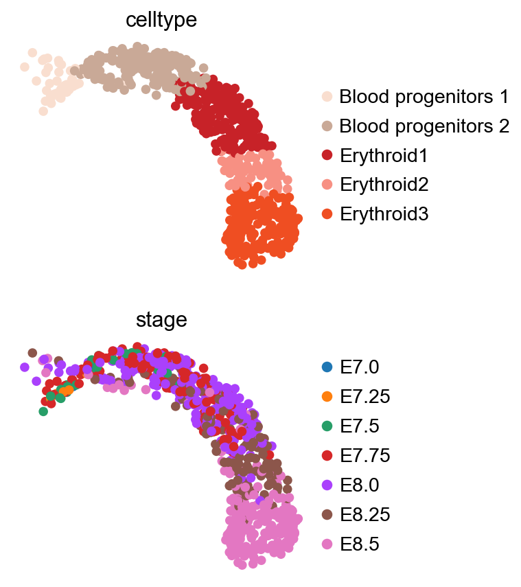
And visualized.

sc.pl.umap(adata, color=["celltype", "stage"], ncols=1)

Pseudotime inference

Pseudotime inference estimates the progression of cells along a continuous trajectory based on their proximity in a low-dimensional space derived from molecular readouts, in this case, gene expression.

It requires a defined starting point, typically based on prior biological knowledge of the tissue under study.

In this case, the trajectory is known to originate from the “Blood Progenitors 1” cell type. The following demonstrates how to infer pseudotime using paga [WHP+19].

Note

In some cases, pseudotime calculation is not necessary, as information about the continuous process of interest may already be available in the metadata or inferred through alternative methods, such as factor scoring in mofacell [RFLD+23].

root_celltype = "Blood progenitors 1"

sc.pp.neighbors(adata, use_rep="X_pca")
sc.tl.diffmap(adata)
sc.pp.neighbors(adata, use_rep="X_diffmap")
sc.tl.paga(adata, groups="celltype")
iroot = np.flatnonzero(adata.obs["celltype"] == root_celltype)[0]
adata.uns["iroot"] = iroot
sc.tl.dpt(adata)

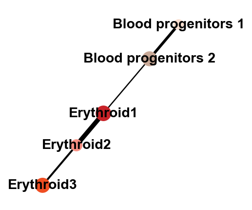
Then, he obtained graph of cell types and the predicted pseudotime can be visualized.

sc.pl.paga(adata, color=["celltype"])
sc.pl.umap(adata, color=["celltype", "dpt_pseudotime"], legend_loc="on data")

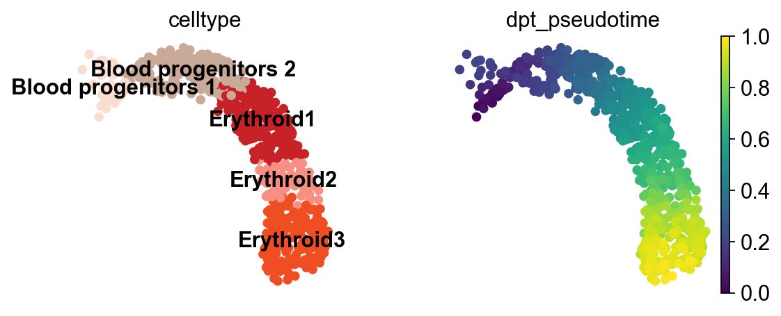
As expected, the predicted pseudotime orders cells from “Blood progenitors 1” to “Erythroid3”.

Enrichment analysis

Enrichment analysis tests whether a specific set of omics features is “overrepresented” or “coordinated” in the measured data compared to a background distribution. These sets are predefined based on existing biological knowledge and may vary depending on the omics technology used.

Enrichment analysis requires the use of an enrichment method, and several options are available. In the original manuscript of decoupler [BiMVSB+22], we benchmarked multiple methods and found that the univariate linear model (ulm) outperformed the others. Therefore, we will use ulm in this vignette.

The scores from decoupler.mt.ulm() should be interpreted such that larger magnitudes indicate greater significance, while the sign reflects whether the features in the set are overrepresented (positive) or underrepresented (negative) compared to the background.

Transcription factor scoring from gene regulatory networks

Transcription factors (TFs) are genes that, once translated into proteins, bind to DNA and regulate the expression of other genes by either promoting or inhibiting their transcription. Gene Regulatory Networks (GRNs) capture these TF-gene interactions and can be constructed from prior knowledge or inferred from omics data. The fundamental unit of a GRN is a TF and its associated target genes, collectively known as a regulon. Each regulon functions as a gene set in enrichment analysis.

Although TFs are measured in transcriptomic data, their transcript levels often do not reflect their actual activity in a given cell. Instead, scoring TFs through enrichment analysis based on the expression of their target genes provides a more accurate representation of their regulatory activity [BiMWMullerD+23].

CollecTRI network

CollecTRI is a comprehensive resource containing a curated collection of TFs and their transcriptional targets compiled from 12 different resources [MullerDTV+23]. This collection provides an increased coverage of transcription factors and a superior performance in identifying perturbed TFs compared to other literature based GRNs such as DoRothEA [GAHI+19]. Similar to DoRothEA, interactions are weighted by their mode of regulation (activation or inhibition).

In this tutorial we will use the mouse version but other organisms are available. We can use decoupler to retrieve it from the OmniPath server [TureiKSR16].

Note In this tutorial we use the network CollecTRI, but we could use any other GRN coming from an inference method such as CellOracle, pySCENIC or SCENIC+.

collectri = dc.op.collectri(organism="mouse")
collectri

	source	target	weight	resources	references	sign_decision
0	Myc	Tert	1.0	DoRothEA-A;ExTRI;HTRI;NTNU.Curated;Pavlidis202...	10022128;10491298;10606235;10637317;10723141;1...	PMID
1	Spi1	Bglap3	1.0	ExTRI	10022617	default activation
2	Spi1	Bglap	1.0	ExTRI	10022617	default activation
3	Spi1	Bglap2	1.0	ExTRI	10022617	default activation
4	Smad3	Jun	1.0	ExTRI;NTNU.Curated;TFactS;TRRUST	10022869;12374795	PMID
...	...	...	...	...	...	...
43221	Runx1	Lcp2	1.0	DoRothEA-A	20019798	default activation
43222	Runx1	Prr5l	1.0	DoRothEA-A	20019798	default activation
43223	Twist1	Gli1	1.0	DoRothEA-A	11948912	default activation
43224	Usf1	Nup188	1.0	DoRothEA-A	22951020	PMID
43225	Zfp148	Rnls	1.0	DoRothEA-A	25295465	PMID

43226 rows × 6 columns

Scoring

TF scores can be easily computed by running the ulm method.

dc.mt.ulm(data=adata, net=collectri)

Scores can then be extracted as a new anndata.AnnData object.

score = dc.pp.get_obsm(adata=adata, key="score_ulm")
score

AnnData object with n_obs × n_vars = 801 × 513
    obs: 'sample', 'stage', 'sequencing.batch', 'theiler', 'celltype', 'dpt_pseudotime'
    uns: 'celltype_colors', 'log1p', 'stage_colors', 'neighbors', 'diffmap_evals', 'paga', 'celltype_sizes', 'iroot'
    obsm: 'X_pca', 'X_umap', 'X_diffmap', 'score_ulm', 'padj_ulm'

And visualized.

tf = "Klf3"
sc.pl.umap(score, color=[tf, "celltype"], cmap="RdBu_r", vcenter=0)
sc.pl.violin(score, keys=[tf], groupby="celltype", rotation=90, ylabel=f"{tf} score")

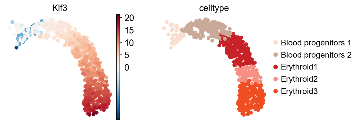
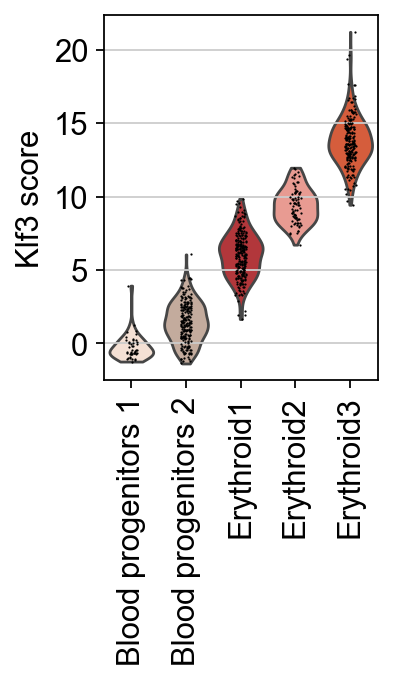
Here, the inferred activity of Klf3 across cells is shown, with an increasing value along the trajectory. Notably, Klf3 is a well-established TF essential in erythroid lineage specification and maturation.

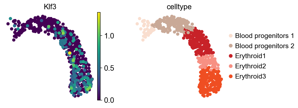
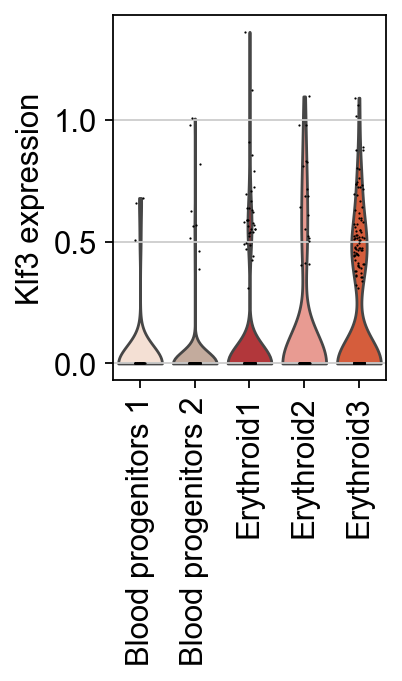
As previously noted, TF expression alone is not a reliable proxy for its activity. For instance, although Klf3 is known to activate during the comitement towards the erythroid lineage, its expression is detected in only a limited number of cells in this dataset. This highlights the importance of using TF enrichment scores.

sc.pl.umap(adata, color=[tf, "celltype"])
sc.pl.violin(adata, keys=[tf], groupby="celltype", rotation=90, ylabel=f"{tf} expression")

Next, TFs associated with the inferred pseudotime can be identified.

tfs = dc.tl.rankby_order(
    adata=score,
    order="dpt_pseudotime",
    stat="dcor",
)
tfs

	name	stat	pval	padj
0	Klf3	1924.545622	0.000000	0.000000
1	Klf1	1802.000715	0.000000	0.000000
2	Hoxb6	1720.184784	0.000000	0.000000
3	Nfe2	1715.817219	0.000000	0.000000
4	Atrx	1562.600819	0.000000	0.000000
...	...	...	...	...
508	Nr0b1	-0.382287	0.648875	0.653975
509	Msc	-0.464131	0.678723	0.682715
510	Rb1	-0.501624	0.692034	0.694742
511	Crx	-0.658420	0.744866	0.746320
512	Ep300	-0.675837	0.750428	0.750428

513 rows × 4 columns

The top 5 TF markers associated to the pseudotime can then be extracted.

top_tfs = tfs.head(5)["name"].to_list()
top_tfs

['Klf3', 'Klf1', 'Hoxb6', 'Nfe2', 'Atrx']

And visualized.

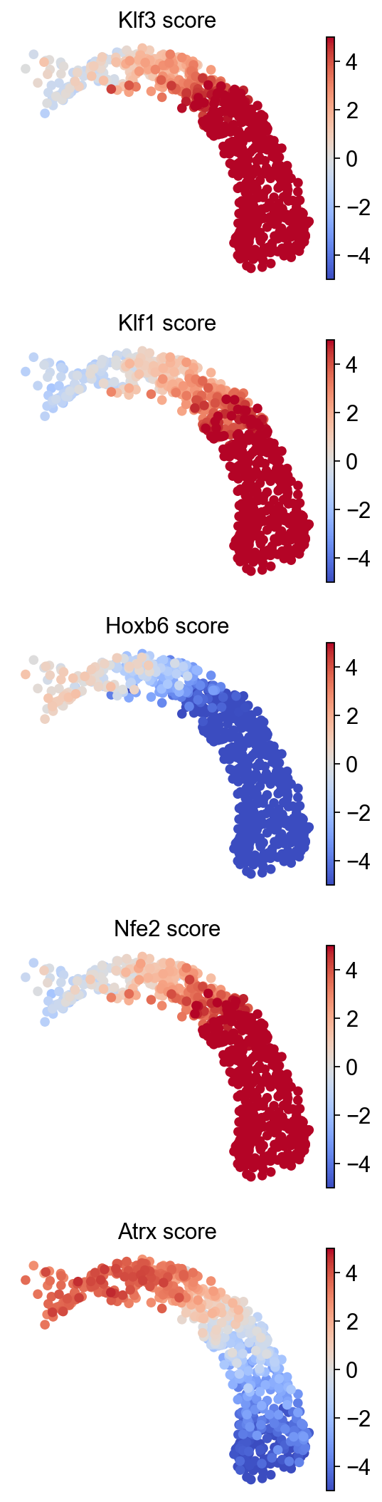
sc.pl.umap(score, color=top_tfs, cmap="coolwarm", vmin=-5, vmax=5, ncols=1, title=[f"{t} score" for t in top_tfs])

Prior to generating more complex visualizations, cells are grouped into bins based on their ordering to facilitate plotting.

bin_tfs = dc.pp.bin_order(
    adata=score,
    order="dpt_pseudotime",
    names=top_tfs,
    label="celltype",
)
bin_tfs

	name	order	value	label	color
0	Klf3	0.005	-1.236535	Blood progenitors 1	#f9decf
1	Klf3	0.005	-0.073794	Blood progenitors 1	#f9decf
2	Klf3	0.005	-0.685060	Blood progenitors 1	#f9decf
3	Klf3	0.005	-0.678414	Blood progenitors 1	#f9decf
4	Klf3	0.015	-0.701368	Blood progenitors 1	#f9decf
...	...	...	...	...	...
4000	Atrx	0.985	-6.894305	Erythroid3	#EF4E22
4001	Atrx	0.985	-4.275815	Erythroid3	#EF4E22
4002	Atrx	0.995	-5.932188	Erythroid3	#EF4E22
4003	Atrx	0.995	-7.659520	Erythroid3	#EF4E22
4004	Atrx	0.995	-9.214737	Erythroid3	#EF4E22

4005 rows × 5 columns

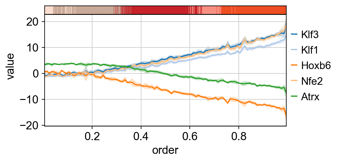
Which can be plotted as lines.

dc.pl.order(
    df=bin_tfs,
    mode="line",
    figsize=(6, 3),
)

Or as a matrix.

dc.pl.order(df=bin_tfs, mode="mat", kw_order={"vmin": -5, "vmax": +5, "cmap": "RdBu_r"}, figsize=(6, 4))

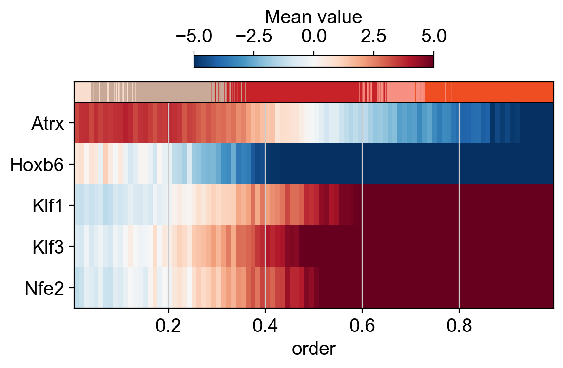
TFs relevant to progenitor cells, such as Atrx and Hoxb6, are active at the beginning of the trajectory. In contrast, TFs involved in commitment to the erythroid lineage, such as the Klf family, are initially inactive but become activated along the trajectory.

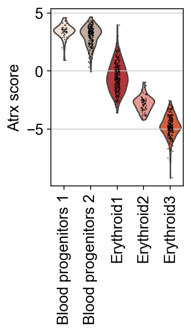
Individual TFs can be examined by plotting their score distributions.

tf = "Atrx"
sc.pl.violin(score, keys=[tf], groupby="celltype", rotation=90, ylabel=f"{tf} score")

Additionally, to better understand the obtained enrichment scores, the targets of a specified TF can be plotted along the trajectory.

dc.pl.order_targets(
    adata=adata,
    net=collectri,
    label="celltype",
    source="Atrx",
    order="dpt_pseudotime",
)

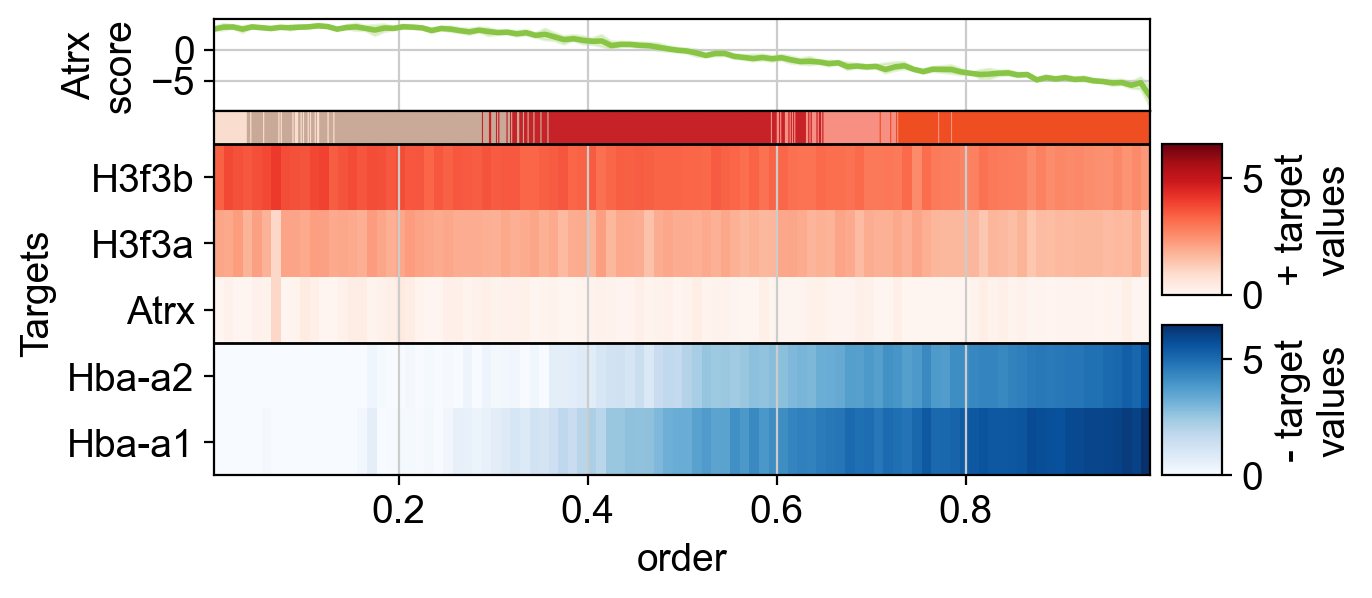
The change in the enrichment score results from positive targets of Atrx decreasing in expression, while its repressed targets increase in expression along the trajectory. Consequently, the TF is active at the beginning but becomes inactive by the end.

Pathway Scoring

The same approach used for TF scoring can also be applied to pathways. Numerous databases provide curated pathway gene sets, with one of the most well-known being MSigDB, which includes several collections [LSP+11]. These and many other resources can be accessed using the function decoupler.op.resource(). To view the list of available databases, use decoupler.op.show_resources().

PROGENy Pathway Genes

PROGENy is a comprehensive resource that provides a curated collection of pathways and their target genes, along with weights for each interaction [SKK+18].

Below is a brief description of each pathway:

• Androgen: involved in the growth and development of the male reproductive organs

• EGFR: regulates growth, survival, migration, apoptosis, proliferation, and differentiation in mammalian cells

• Estrogen: promotes the growth and development of the female reproductive organs

• Hypoxia: promotes angiogenesis and metabolic reprogramming when O2 levels are low

• JAK-STAT: involved in immunity, cell division, cell death, and tumor formation

• MAPK: integrates external signals and promotes cell growth and proliferation

• NFkB: regulates immune response, cytokine production and cell survival

• p53: regulates cell cycle, apoptosis, DNA repair and tumor suppression

• PI3K: promotes growth and proliferation

• TGFb: involved in development, homeostasis, and repair of most tissues

• TNFa: mediates haematopoiesis, immune surveillance, tumour regression and protection from infection

• Trail: induces apoptosis

• VEGF: mediates angiogenesis, vascular permeability, and cell migration

• WNT: regulates organ morphogenesis during development and tissue repair

This is how to access to it.

progeny = dc.op.progeny(organism="mouse")
progeny

	source	target	weight	padj
0	Androgen	Tmprss2	11.490631	2.384806e-47
1	Androgen	Nkx3-1	10.622551	2.205102e-44
2	Androgen	Mboat2	10.472733	4.632376e-44
3	Androgen	Slc38a4	7.363805	1.253071e-39
4	Androgen	Mtmr9	6.130646	2.534403e-38
...	...	...	...	...
60572	p53	Enpp2	2.771405	4.993215e-02
60573	p53	Arrdc4	3.494328	4.996747e-02
60574	p53	Myo1b	-1.148057	4.997905e-02
60575	p53	Ctsc	-1.784693	4.998864e-02
60576	p53	Naa50	-1.435013	4.998884e-02

60577 rows × 4 columns

Scoring

Pathway scores can be easily computed by running the ulm method.

dc.mt.ulm(data=adata, net=progeny)

Scores can then be extracted.

score = dc.pp.get_obsm(adata=adata, key="score_ulm")
score

AnnData object with n_obs × n_vars = 801 × 14
    obs: 'sample', 'stage', 'sequencing.batch', 'theiler', 'celltype', 'dpt_pseudotime'
    uns: 'celltype_colors', 'log1p', 'stage_colors', 'neighbors', 'diffmap_evals', 'paga', 'celltype_sizes', 'iroot'
    obsm: 'X_pca', 'X_umap', 'X_diffmap', 'score_ulm', 'padj_ulm'

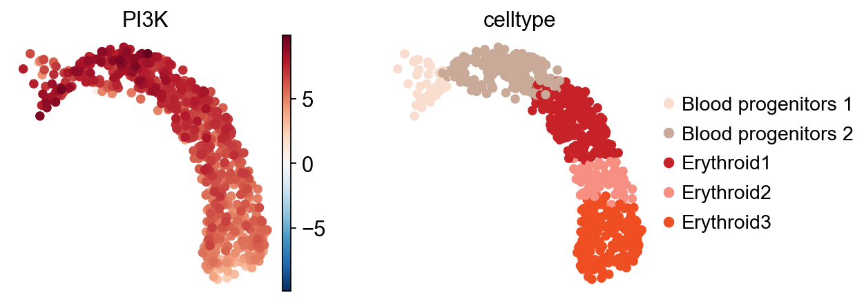
And visualized.

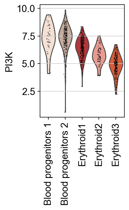
sc.pl.umap(score, color=["PI3K", "celltype"], cmap="RdBu_r", vcenter=0)
sc.pl.violin(score, keys=["PI3K"], groupby="celltype", rotation=90)

Next, the association between pathways and the trajectory can be tested.

pws = dc.tl.rankby_order(
    adata=score,
    order="dpt_pseudotime",
)
pws

	name	stat	pval	padj
0	PI3K	332.077288	0.000000e+00	0.000000e+00
1	EGFR	292.234849	0.000000e+00	0.000000e+00
2	MAPK	271.986785	0.000000e+00	0.000000e+00
3	VEGF	118.975377	0.000000e+00	0.000000e+00
4	TGFb	102.538265	0.000000e+00	0.000000e+00
5	Estrogen	100.245675	0.000000e+00	0.000000e+00
6	p53	84.836576	0.000000e+00	0.000000e+00
7	WNT	81.348290	0.000000e+00	0.000000e+00
8	NFkB	74.053878	0.000000e+00	0.000000e+00
9	TNFa	55.833994	0.000000e+00	0.000000e+00
10	JAK-STAT	46.853171	0.000000e+00	0.000000e+00
11	Trail	45.698393	0.000000e+00	0.000000e+00
12	Hypoxia	7.035028	9.980905e-13	1.074867e-12
13	Androgen	3.231894	6.149262e-04	6.149262e-04

And plotted.

bin_pws = dc.pp.bin_order(
    adata=score,
    order="dpt_pseudotime",
    names=pws.head(5)["name"].to_list(),
    label="celltype",
)
bin_pws

	name	order	value	label	color
0	PI3K	0.005	9.238632	Blood progenitors 1	#f9decf
1	PI3K	0.005	7.656678	Blood progenitors 1	#f9decf
2	PI3K	0.005	7.569328	Blood progenitors 1	#f9decf
3	PI3K	0.005	6.936269	Blood progenitors 1	#f9decf
4	PI3K	0.015	8.850726	Blood progenitors 1	#f9decf
...	...	...	...	...	...
4000	TGFb	0.985	-2.011171	Erythroid3	#EF4E22
4001	TGFb	0.985	-3.271655	Erythroid3	#EF4E22
4002	TGFb	0.995	-2.304044	Erythroid3	#EF4E22
4003	TGFb	0.995	-2.470572	Erythroid3	#EF4E22
4004	TGFb	0.995	-2.429676	Erythroid3	#EF4E22

4005 rows × 5 columns

dc.pl.order(df=bin_pws, mode="mat", kw_order={"vmin": -10, "vmax": +10, "cmap": "RdBu_r"}, figsize=(6, 3))

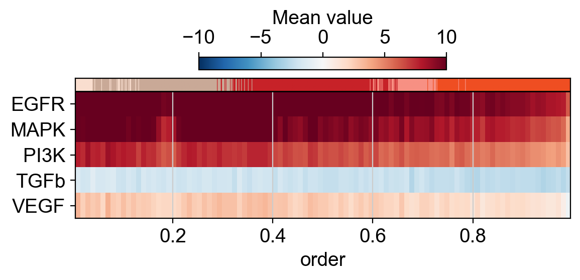
It seems that along the trajectory there are no big changes, just a mild decrease of PI3K activity.

Hallmark gene sets

Hallmark gene sets are curated collections of genes that represent specific, well-defined biological states or processes. They are part of MSigDB and were developed to reduce redundancy and improve interpretability compared to older, more overlapping gene set collections [LSP+11].

A total of 50 gene sets are provided, designed to be non-redundant, concise, and biologically coherent.

This is how to access them.

hallmark = dc.op.hallmark(organism="mouse")
hallmark

	source	target
0	IL2_STAT5_SIGNALING	Maff
1	COAGULATION	Maff
2	HYPOXIA	Maff
3	TNFA_SIGNALING_VIA_NFKB	Maff
4	COMPLEMENT	Maff
...	...	...
7606	PANCREAS_BETA_CELLS	Stxbp1
7607	PANCREAS_BETA_CELLS	Elp4
7608	PANCREAS_BETA_CELLS	Gcg
7609	PANCREAS_BETA_CELLS	Pcsk2
7610	PANCREAS_BETA_CELLS	Pax6

7611 rows × 2 columns

Scoring

Pathway scores can be easily computed by running the ulm method.

dc.mt.ulm(data=adata, net=hallmark)

Scores can be then extracted.

score = dc.pp.get_obsm(adata=adata, key="score_ulm")
score

AnnData object with n_obs × n_vars = 801 × 50
    obs: 'sample', 'stage', 'sequencing.batch', 'theiler', 'celltype', 'dpt_pseudotime'
    uns: 'celltype_colors', 'log1p', 'stage_colors', 'neighbors', 'diffmap_evals', 'paga', 'celltype_sizes', 'iroot'
    obsm: 'X_pca', 'X_umap', 'X_diffmap', 'score_ulm', 'padj_ulm'

Tested for association to the trajectory.

hlm = dc.tl.rankby_order(
    adata=score,
    order="dpt_pseudotime",
)
hlm.head()

	name	stat	pval	padj
0	HEME_METABOLISM	1490.562975	0.0	0.0
1	SPERMATOGENESIS	380.618295	0.0	0.0
2	EPITHELIAL_MESENCHYMAL_TRANSITION	307.059413	0.0	0.0
3	APICAL_JUNCTION	287.575912	0.0	0.0
4	ADIPOGENESIS	280.456456	0.0	0.0

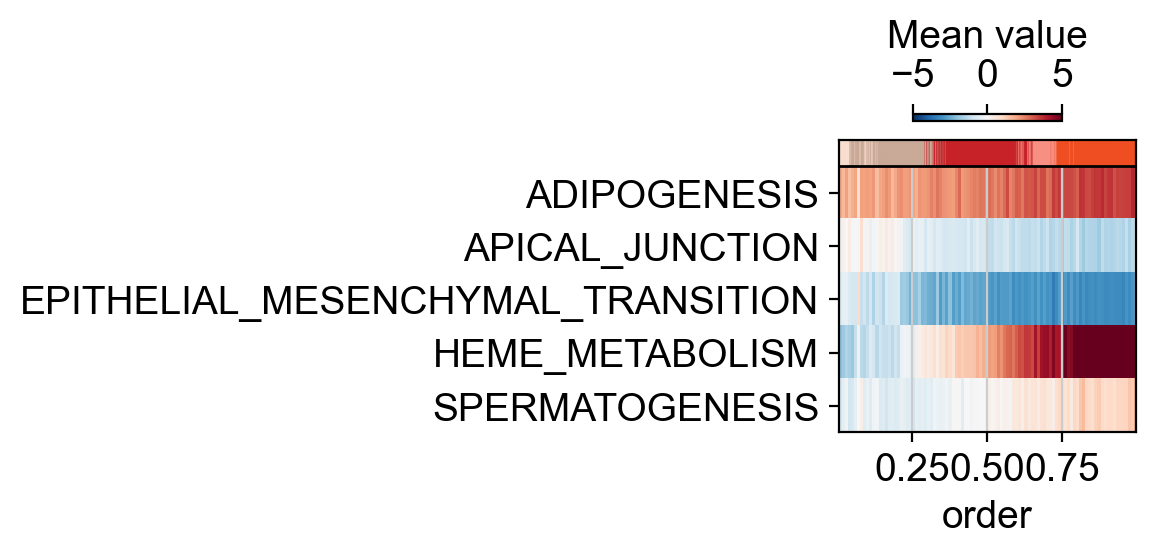
And plotted.

bin_hlm = dc.pp.bin_order(
    adata=score,
    order="dpt_pseudotime",
    names=hlm.head(5)["name"].to_list(),
    label="celltype",
)
bin_hlm

	name	order	value	label	color
0	HEME_METABOLISM	0.005	-1.584656	Blood progenitors 1	#f9decf
1	HEME_METABOLISM	0.005	-3.012170	Blood progenitors 1	#f9decf
2	HEME_METABOLISM	0.005	-1.934134	Blood progenitors 1	#f9decf
3	HEME_METABOLISM	0.005	-1.641200	Blood progenitors 1	#f9decf
4	HEME_METABOLISM	0.015	-1.550928	Blood progenitors 1	#f9decf
...	...	...	...	...	...
4000	ADIPOGENESIS	0.985	3.631165	Erythroid3	#EF4E22
4001	ADIPOGENESIS	0.985	4.255289	Erythroid3	#EF4E22
4002	ADIPOGENESIS	0.995	3.177657	Erythroid3	#EF4E22
4003	ADIPOGENESIS	0.995	3.437600	Erythroid3	#EF4E22
4004	ADIPOGENESIS	0.995	4.256072	Erythroid3	#EF4E22

4005 rows × 5 columns

dc.pl.order(df=bin_hlm, mode="mat", kw_order={"vmin": -5, "vmax": +5, "cmap": "RdBu_r"}, figsize=(6, 3))