Single-cell Enrichment Analysis

Single-cell RNA-seq (scRNA-seq) yields many molecular readouts that are hard to interpret by themselves. One common approach to summarize this data is to compute enrichment scores using predefined gene sets based on prior biological knowledge.

In this notebook, we demonstrate how to use decoupler to infer transcription factor (TF) and pathway enrichment scores from a scRNA-seq human dataset.

The dataset includes 3k peripheral blood mononuclear cells (PBMCs) from a healthy donor. It publicly available at the 10x Genomics webpage.

Note

When your data consist of different conditions with multiple samples (patients, mice, etc.), it is recommended to use pseudobulk profiles instead

Loading Packages

import scanpy as sc
import decoupler as dc

sc.set_figure_params(figsize=(3, 3), frameon=False)

Loading The Dataset

adata = dc.ds.pbmc3k()
adata

AnnData object with n_obs × n_vars = 2638 × 13714
    obs: 'n_genes', 'percent_mito', 'n_counts', 'celltype', 'leiden'
    var: 'n_cells'
    uns: 'draw_graph', 'louvain', 'louvain_colors', 'neighbors', 'pca', 'rank_genes_groups'
    obsm: 'X_pca', 'X_tsne', 'X_umap', 'X_draw_graph_fr'
    obsp: 'distances', 'connectivities'

The obtained anndata.AnnData consist of log-normalized transcript counts for ~3k cells with measurements for ~15k genes.

The cell metadata stored in anndata.AnnData.obs can be inspected.

adata.obs

	n_genes	percent_mito	n_counts	celltype	leiden
index
AAACATACAACCAC-1	781	0.030178	2419.0	CD4 T cells	Clust:0
AAACATTGAGCTAC-1	1352	0.037936	4903.0	B cells	Clust:2
AAACATTGATCAGC-1	1131	0.008897	3147.0	CD4 T cells	Clust:0
AAACCGTGCTTCCG-1	960	0.017431	2639.0	CD14+ Monocytes	Clust:1
AAACCGTGTATGCG-1	522	0.012245	980.0	NK cells	Clust:4
...	...	...	...	...	...
TTTCGAACTCTCAT-1	1155	0.021104	3459.0	CD14+ Monocytes	Clust:1
TTTCTACTGAGGCA-1	1227	0.009294	3443.0	B cells	Clust:2
TTTCTACTTCCTCG-1	622	0.021971	1684.0	B cells	Clust:2
TTTGCATGAGAGGC-1	454	0.020548	1022.0	B cells	Clust:2
TTTGCATGCCTCAC-1	724	0.008065	1984.0	CD4 T cells	Clust:0

2638 rows × 5 columns

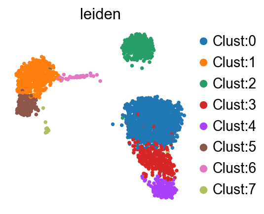
And visualized.

sc.pl.umap(
    adata=adata,
    color="leiden",
)

Enrichment analysis

Enrichment analysis tests whether a specific set of omics features is “overrepresented” or “coordinated” in the measured data compared to a background distribution. These sets are predefined based on existing biological knowledge and may vary depending on the omics technology used.

Enrichment analysis requires the use of an enrichment method, and several options are available. In the original manuscript of decoupler [BiMVSB+22], we benchmarked multiple methods and found that the univariate linear model (ulm) outperformed the others. Therefore, we will use ulm in this vignette.

The scores from decoupler.mt.ulm() should be interpreted such that larger magnitudes indicate greater significance, while the sign reflects whether the features in the set are overrepresented (positive) or underrepresented (negative) compared to the background.

Cell type scoring based on marker genes

In single-cell analysis, there is no measured readout that directly informs about the cell type of each individual cell. To assign cell type labels, cells are first projected into a shared embedded space. Through clustering, groups of cells with similar transcriptional profiles are then identified, and the expression of known cell type-specific markers are used to annotate the cells. These markers, identified and annotated in previous studies, are collected and curated in various reference resources. When multiple marker genes are available, enrichment methods can be used to score marker sets within cells, providing guidance for annotating the resulting clusters.

PanglaoDB

PanglaoDB [FGBjorkegren19] is a database that compiles and annotates cell type markers across multiple tissues. It can be conveniently accessed through the OmniPath module of decoupler [TureiKSR16].

Note

Other cell marker databases are avaliable, such as CellTypist, which can be accessed with the same function decoupler.op.resource

markers = dc.op.resource("PanglaoDB", organism="human")
markers

	genesymbol	canonical_marker	cell_type	germ_layer	human	human_sensitivity	human_specificity	mouse	mouse_sensitivity	mouse_specificity	ncbi_tax_id	organ	ubiquitiousness
0	A0A068BD53	True	B cells	Mesoderm	False	0.000000	0.000000	True	0.391473	0.002740	10090	Immune system	0.007
1	A0A068BGV1	True	Dendritic cells	Mesoderm	False	0.000000	0.000000	True	0.142857	0.000193	10090	Immune system	0.000
2	A0A068BGW6	True	B cells	Mesoderm	False	0.000000	0.000000	True	0.391473	0.002740	10090	Immune system	0.007
3	A0A087WRN7	False	Salivary mucous cells	Ectoderm	False	NaN	NaN	True	NaN	NaN	10090	Oral cavity	0.001
4	A0A0F6QAG2	True	NK cells	Mesoderm	False	0.000000	0.000000	True	0.372340	0.000129	10090	Immune system	0.002
...	...	...	...	...	...	...	...	...	...	...	...	...	...
8456	ZNF521	False	Adipocyte progenitor cells	Mesoderm	True	0.000000	0.010338	False	0.000000	0.000000	9606	Connective tissue	0.002
8457	ZNRF4	False	Germ cells	Mesoderm	True	0.284360	0.000000	True	0.000000	0.000000	9606	Reproductive	0.010
8458	ZPBP2	True	Germ cells	Mesoderm	True	0.436019	0.000000	True	0.000000	0.000000	9606	Reproductive	0.008
8459	ZRSR2P1	False	Neurons	Ectoderm	True	0.000000	0.000000	True	0.000000	0.000000	9606	Brain	0.005
8460	ZSCAN10	False	Embryonic stem cells	Epiblast	True	0.000000	0.000313	True	0.000000	0.000000	9606	Zygote	0.000

8461 rows × 13 columns

Since the dataset consists of human cells and high-quality markers are preferred, the markers can be filtered to retain only those labeled as canonical and specific to human.

We also format the network of gene sets into the decoupler format: source, target

# Filter by canonical_marker and human
markers = markers[
    markers["human"].astype(bool)
    & markers["canonical_marker"].astype(bool)
    & (markers["human_sensitivity"].astype(float) > 0.5)
]

# Remove duplicated entries
markers = markers[~markers.duplicated(["cell_type", "genesymbol"])]

# Format
markers = markers.rename(columns={"cell_type": "source", "genesymbol": "target"})
markers = markers[["source", "target"]]
markers

	source	target
50	Pulmonary alveolar type II cells	ABCA3
122	Enterocytes	ACSL5
133	Smooth muscle cells	ACTA2
144	Myoepithelial cells	ACTG2
145	Smooth muscle cells	ACTG2
...	...	...
8341	Endothelial cells	VWF
8350	Luminal epithelial cells	WFDC2
8351	Ductal cells	WFDC2
8380	Podocytes	WT1
8447	Ependymal cells	ZMYND10

691 rows × 2 columns

In this tutorial, these markers will be used, but any gene collection could be applied, including custom gene sets.

Scoring

We can easily compute cell type enrichment scores by running the ulm method.

dc.mt.ulm(data=adata, net=markers, tmin=3)

The obtained scores (score_ulm) and adjusted p-values (padj_ulm) were stored in the adata.obsm keys.

adata.obsm["score_ulm"]

	Acinar cells	Adipocytes	Alpha cells	B cells	B cells naive	Dendritic cells	Ductal cells	Endothelial cells	Enterocytes	Ependymal cells	...	Pancreatic stellate cells	Pericytes	Plasma cells	Plasmacytoid dendritic cells	Platelets	Podocytes	Proximal tubule cells	Pulmonary alveolar type II cells	Smooth muscle cells	T cells
AAACATACAACCAC-1	-0.574614	0.880015	1.501143	4.869608	3.822776	7.993952	-0.406252	-0.908959	-0.454221	-0.406252	...	-0.351811	1.501143	3.070459	0.325694	4.707824	-0.574614	-0.574614	-0.497593	-0.454221	13.437334
AAACATTGAGCTAC-1	-0.752534	-0.266765	0.907750	10.639314	12.676054	14.592025	2.193505	0.266856	0.217661	-0.532039	...	-0.460741	2.193505	6.653792	1.056778	3.699963	-0.752534	-0.752534	-0.651663	-0.594861	3.827107
AAACATTGATCAGC-1	-0.717204	0.775482	1.195078	3.379488	6.287648	7.469071	-0.507061	-0.018701	-0.566934	-0.507061	...	-0.439111	2.715337	1.806525	-0.318529	6.199206	-0.717204	0.042273	-0.621069	-0.566934	15.211887
AAACCGTGCTTCCG-1	0.614963	2.143531	0.671311	8.120865	4.465337	26.901402	1.338112	0.568580	-0.523795	0.671311	...	-0.405698	0.671311	4.233656	0.420052	7.887647	0.143440	-0.662630	-0.573810	-0.523795	5.473293
AAACCGTGTATGCG-1	-0.498060	-0.556890	1.495823	2.115894	0.170480	15.537294	-0.352129	0.039016	-0.393707	-0.352129	...	-0.304941	-0.352129	0.703835	3.160296	6.316497	-0.498060	-0.498060	-0.431300	-0.393707	3.873352
...	...	...	...	...	...	...	...	...	...	...	...	...	...	...	...	...	...	...	...	...	...
TTTCGAACTCTCAT-1	1.131347	1.491715	1.096136	7.689370	3.972790	26.218950	2.529991	1.203758	-0.569493	-0.509350	...	-0.441093	2.702240	4.672744	1.096436	5.488147	-0.720441	-0.720441	-0.623872	-0.569493	5.171710
TTTCTACTGAGGCA-1	-0.745205	-0.833229	1.081317	9.558244	5.570785	12.581891	2.096218	-0.270738	-0.589067	-0.526857	...	-0.456254	2.984098	13.259767	2.046399	5.558045	-0.745205	-0.745205	-0.645316	-0.589067	2.361846
TTTCTACTTCCTCG-1	-0.525565	-0.587644	1.020571	15.879073	15.877780	17.799659	-0.371575	-0.831368	-0.415449	-0.371575	...	-0.321781	-0.371575	8.865448	1.326769	4.018225	-0.525565	-0.525565	-0.455119	-0.415449	4.885653
TTTGCATGAGAGGC-1	-0.459498	-0.513773	-0.324865	20.431676	15.533753	19.685476	-0.324865	-0.726856	-0.363224	-0.324865	...	-0.281331	-0.324865	8.988557	1.406361	4.553272	-0.459498	-0.459498	-0.397907	-0.363224	5.776182
TTTGCATGCCTCAC-1	-0.560244	-0.626420	-0.396092	2.206213	4.451617	9.228275	1.670463	0.621853	-0.442862	-0.396092	...	-0.343013	0.907680	-0.594251	0.732566	3.389654	-0.560244	-0.560244	-0.485149	-0.442862	12.191711

2638 rows × 36 columns

To visualize the obtained scores, we can re-use many of scanpy’s plotting functions. First though, we need to extract them from the adata object.

score = dc.pp.get_obsm(adata, key="score_ulm")
score

AnnData object with n_obs × n_vars = 2638 × 36
    obs: 'n_genes', 'percent_mito', 'n_counts', 'celltype', 'leiden'
    uns: 'draw_graph', 'louvain', 'louvain_colors', 'neighbors', 'pca', 'rank_genes_groups', 'leiden_colors'
    obsm: 'X_pca', 'X_tsne', 'X_umap', 'X_draw_graph_fr', 'score_ulm', 'padj_ulm'

decoupler.pp.get_obsm() returns a new anndata.AnnData object which holds the obtained activities in its anndata.AnnData.X attribute.

sc.pl.umap(score, color=["NK cells", "leiden"], cmap="RdBu_r")
sc.pl.violin(score, keys=["NK cells"], groupby="leiden", rotation=90)

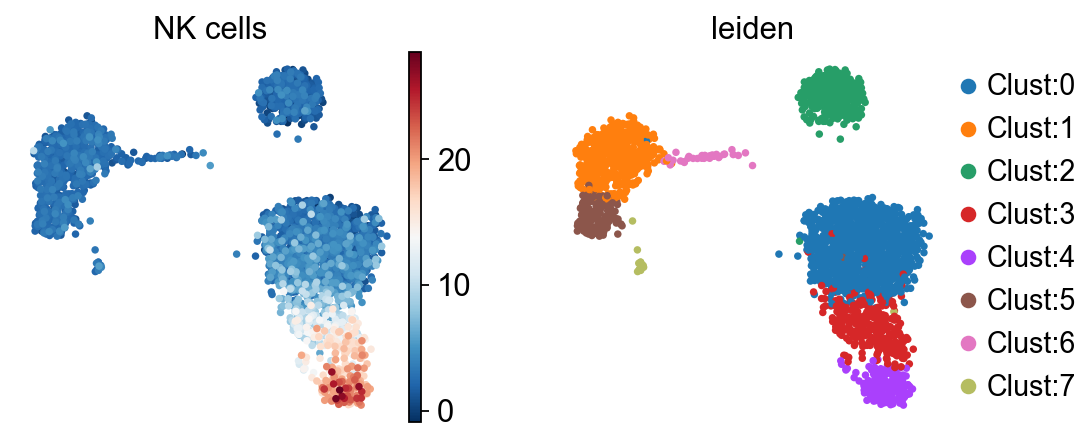
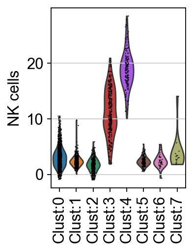
The highlighted cells appear to be enriched for NK cell marker genes, with most of them belonging to cluster 4 or 3.

With decoupler, the top predicted cell types per cluster can also be identified using the function decoupler.tl.rankby_group(). This function identifies “marker” cell types per cluster using the same statistical tests available in scanpy.tl.rank_genes_groups().

df = dc.tl.rankby_group(adata=score, groupby="leiden", reference="rest", method="t-test_overestim_var")
df = df[df["stat"] > 0]
df

	group	reference	name	stat	meanchange	pval	padj
1	Clust:0	rest	T cells	38.206923	4.718293	5.308180e-247	9.554725e-246
22	Clust:0	rest	Neurons	6.885109	0.195677	7.446037e-12	1.165467e-11
23	Clust:0	rest	Erythroid-like and erythroid precursor cells	6.733126	0.211885	2.096498e-11	3.144747e-11
27	Clust:0	rest	Oligodendrocytes	3.551632	0.077581	3.905947e-04	5.021931e-04
28	Clust:0	rest	Pericytes	3.514299	0.194079	4.497034e-04	5.582525e-04
...	...	...	...	...	...	...	...
282	Clust:7	rest	Gamma delta T cells	0.438223	0.729249	6.656753e-01	7.730423e-01
283	Clust:7	rest	Alpha cells	0.297565	0.133760	7.682714e-01	8.285775e-01
285	Clust:7	rest	Neurons	0.278680	0.067593	7.825454e-01	8.285775e-01
286	Clust:7	rest	Luminal epithelial cells	0.220853	0.123104	8.268214e-01	8.504448e-01
287	Clust:7	rest	Fibroblasts	0.173151	0.101706	8.639469e-01	8.639469e-01

133 rows × 7 columns

The top 3 predicted cell types per cluster can then be extracted.

n_ctypes = 3
ctypes_dict = df.groupby("group").head(n_ctypes).groupby("group")["name"].apply(lambda x: list(x)).to_dict()
ctypes_dict

{'Clust:0': ['T cells',
  'Neurons',
  'Erythroid-like and erythroid precursor cells'],
 'Clust:1': ['Neutrophils', 'Monocytes', 'Dendritic cells'],
 'Clust:2': ['B cells', 'B cells naive', 'Plasma cells'],
 'Clust:3': ['NK cells', 'Gamma delta T cells', 'T cells'],
 'Clust:4': ['Gamma delta T cells',
  'NK cells',
  'Plasmacytoid dendritic cells'],
 'Clust:5': ['Macrophages', 'Dendritic cells', 'Monocytes'],
 'Clust:6': ['Dendritic cells', 'Luminal epithelial cells', 'Ductal cells'],
 'Clust:7': ['Platelets', 'Endothelial cells', 'Hepatic stellate cells']}

The obtained top predicted cell types can be visualized.

sc.pl.matrixplot(
    adata=score,
    var_names=ctypes_dict,
    groupby="leiden",
    dendrogram=True,
    standard_scale="var",
    colorbar_title="Z-scaled scores",
    cmap="RdBu_r",
)

WARNING: dendrogram data not found (using key=dendrogram_leiden). Running `sc.tl.dendrogram` with default parameters. For fine tuning it is recommended to run `sc.tl.dendrogram` independently.

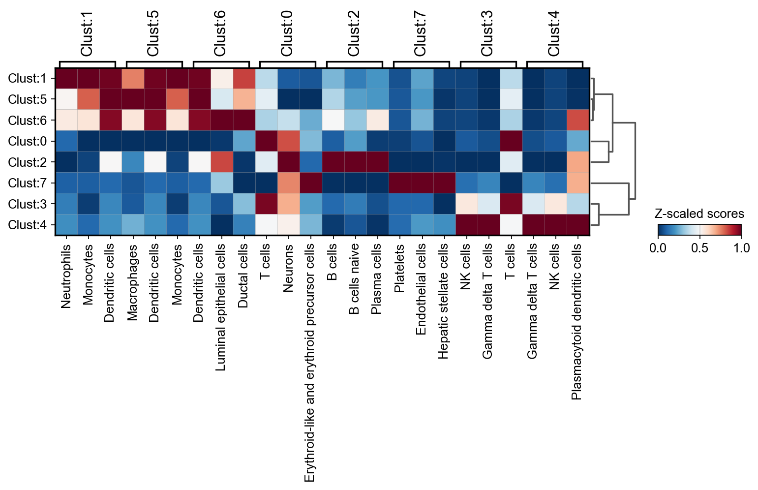
The plot reveals that cluster 7 corresponds to Platelets, cluster 4 appears to be NK cells, clusters 0 and 3 may represent T-cells, cluster 2 is likely a form of B cells, and clusters 6, 5, and 1 belong to the myeloid lineage.

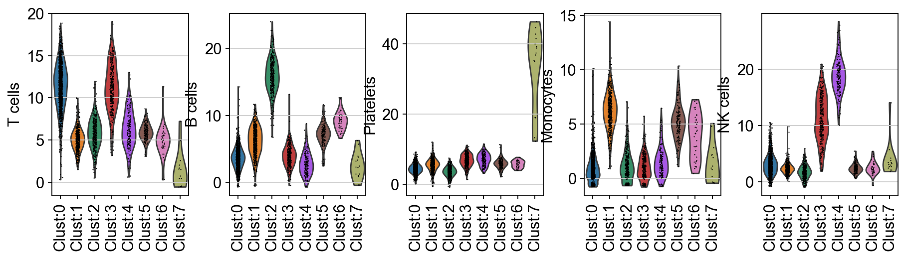
Individual cell types can be examined by plotting their distributions.sc.pl.violin(acts, keys=[‘T cells’, ‘B cells’, ‘Platelets’, ‘Monocytes’, ‘NK cells’], groupby=’leiden’)

sc.pl.violin(
    adata=score,
    keys=["T cells", "B cells", "Platelets", "Monocytes", "NK cells"],
    groupby="leiden",
    rotation=90,
)

Final annotation should be performed manually based on the interpretation of enrichment results. However, an automatic prediction can be generated by assigning the top predicted cell type to each cluster. Although this approach does not require tissue-specific expertise, it may lead to inaccuracies. Nevertheless, it can serve as a useful starting point.

dict_ann = df[df["stat"] > 0].groupby("group").head(1).set_index("group")["name"].to_dict()
dict_ann

{'Clust:0': 'T cells',
 'Clust:2': 'B cells',
 'Clust:1': 'Neutrophils',
 'Clust:4': 'Gamma delta T cells',
 'Clust:3': 'NK cells',
 'Clust:5': 'Macrophages',
 'Clust:6': 'Dendritic cells',
 'Clust:7': 'Platelets'}

Once the top cell type has been selected for each cluster, annotation can be performed.

# Update cats
adata.obs["leiden"] = adata.obs["leiden"].cat.rename_categories(dict_ann)

In this case, the predicted annotations can also be compared to the known reference annotations

sc.pl.umap(
    adata=adata,
    color=["celltype", "leiden"],
    ncols=1,
)

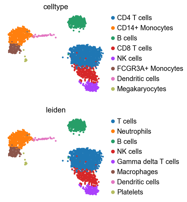
Compared to the original annotation from the scanpy tutorial [WAT18], the results are largely similar, though some discrepancies are present, highlighting the limitations of automatic annotation.

While automatic methods are effective for identifying general lineages, they may be less reliable when distinguishing specific cell type subsets.

Therefore, cell annotation should always be reviewed by a domain expert familiar with the tissue of interest. This section only illustrates how to generate an initial draft annotation. The remainder of the tutorial will use the reference annotations.

Transcription factor scoring from gene regulatory networks

Transcription factors (TFs) are genes that, once translated into proteins, bind to DNA and regulate the expression of other genes by either promoting or inhibiting their transcription. Gene Regulatory Networks (GRNs) capture these TF-gene interactions and can be constructed from prior knowledge or inferred from omics data. The fundamental unit of a GRN is a TF and its associated target genes, collectively known as a regulon. Each regulon functions as a gene set in enrichment analysis.

Although TFs are measured in transcriptomic data, their transcript levels often do not reflect their actual activity in a given cell. Instead, scoring TFs through enrichment analysis based on the expression of their target genes provides a more accurate representation of their regulatory activity [BiMWMullerD+23].

CollecTRI network

CollecTRI is a comprehensive resource containing a curated collection of TFs and their transcriptional targets compiled from 12 different resources [MullerDTV+23]. This collection provides an increased coverage of transcription factors and a superior performance in identifying perturbed TFs compared to other literature based GRNs such as DoRothEA [GAHI+19]. Similar to DoRothEA, interactions are weighted by their mode of regulation (activation or inhibition).

In this tutorial we will use the human version but other organisms are available. We can use decoupler to retrieve it from the OmniPath server [TureiKSR16].

Note

In this tutorial we use the network CollecTRI, but we could use any other GRN coming from an inference method such as CellOracle, pySCENIC or SCENIC+.

collectri = dc.op.collectri(organism="human")
collectri

	source	target	weight	resources	references	sign_decision
0	MYC	TERT	1.0	DoRothEA-A;ExTRI;HTRI;NTNU.Curated;Pavlidis202...	10022128;10491298;10606235;10637317;10723141;1...	PMID
1	SPI1	BGLAP	1.0	ExTRI	10022617	default activation
2	SMAD3	JUN	1.0	ExTRI;NTNU.Curated;TFactS;TRRUST	10022869;12374795	PMID
3	SMAD4	JUN	1.0	ExTRI;NTNU.Curated;TFactS;TRRUST	10022869;12374795	PMID
4	STAT5A	IL2	1.0	ExTRI	10022878;11435608;17182565;17911616;22854263;2...	default activation
...	...	...	...	...	...	...
42985	NFKB	hsa-miR-143-3p	1.0	ExTRI	19472311	default activation
42986	AP1	hsa-miR-206	1.0	ExTRI;GEREDB;NTNU.Curated	19721712	PMID
42987	NFKB	hsa-miR-21	1.0	ExTRI	20813833;22387281	default activation
42988	NFKB	hsa-miR-224-5p	1.0	ExTRI	23474441;23988648	default activation
42989	AP1	hsa-miR-144-3p	1.0	ExTRI	23546882	default activation

42990 rows × 6 columns

Scoring

TF scores can be easily computed by running the ulm method.

dc.mt.ulm(data=adata, net=collectri)

Scores can be then extracted.

score = dc.pp.get_obsm(adata=adata, key="score_ulm")
score

AnnData object with n_obs × n_vars = 2638 × 606
    obs: 'n_genes', 'percent_mito', 'n_counts', 'celltype', 'leiden'
    uns: 'draw_graph', 'louvain', 'louvain_colors', 'neighbors', 'pca', 'rank_genes_groups', 'leiden_colors', 'dendrogram_leiden', 'celltype_colors'
    obsm: 'X_pca', 'X_tsne', 'X_umap', 'X_draw_graph_fr', 'score_ulm', 'padj_ulm'

And visualized.

tf = "PAX5"
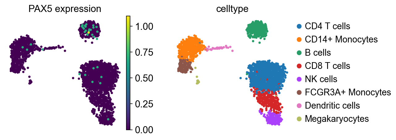
sc.pl.umap(score, color=[tf, "celltype"], cmap="RdBu_r", vcenter=0, title=[f"{tf} score", "celltype"])
sc.pl.violin(score, keys=[tf], groupby="celltype", rotation=90, ylabel=f"{tf} score")

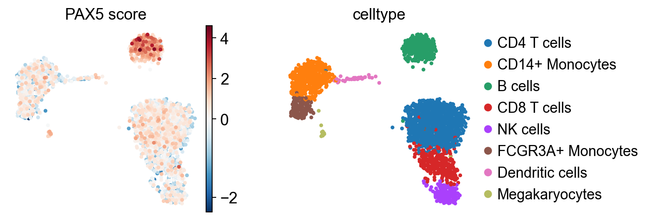
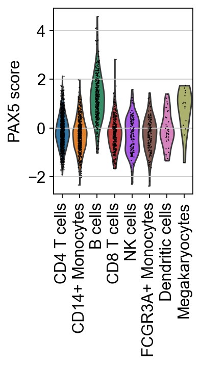
Here, the inferred activity of PAX5 across cells is shown, with particularly high activity in B cells. Notably, PAX5 is a well-established TF essential for B cell identity and function [CSDB07].

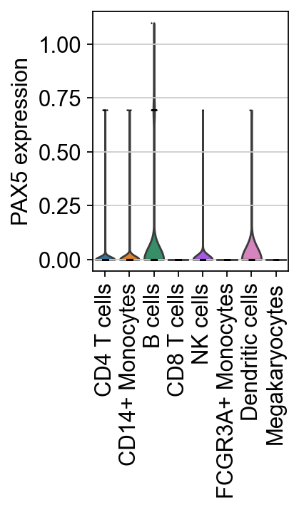
As previously noted, TF expression alone is not a reliable proxy for its activity. For instance, although PAX5 is known to be active in B cells, its expression is detected in only a limited number of cells in this dataset. This highlights the importance of using TF enrichment scores.

sc.pl.umap(adata, color=[tf, "celltype"], title=[f"{tf} expression", "celltype"])
sc.pl.violin(adata, keys=[tf], groupby="celltype", rotation=90, ylabel=f"{tf} expression")

Next, marker TFs for each cell type can be identified.

df = dc.tl.rankby_group(adata=score, groupby="celltype", reference="rest", method="t-test_overestim_var")
df = df[df["stat"] > 0]
df

	group	reference	name	stat	meanchange	pval	padj
9	CD4 T cells	rest	ZBTB4	33.614919	2.688046	1.054929e-195	6.392872e-194
11	CD4 T cells	rest	MYC	31.367690	2.156232	1.369677e-171	6.916871e-170
28	CD4 T cells	rest	ZBED1	24.925535	1.379326	9.114879e-121	1.904695e-119
29	CD4 T cells	rest	KLF3	24.540906	1.130052	3.574529e-118	7.220548e-117
43	CD4 T cells	rest	TRERF1	21.797367	0.628027	1.835785e-95	2.528377e-94
...	...	...	...	...	...	...	...
4840	Megakaryocytes	rest	SIM2	0.018855	0.005540	9.850910e-01	9.966029e-01
4841	Megakaryocytes	rest	TRERF1	0.012646	0.002931	9.900187e-01	9.974627e-01
4843	Megakaryocytes	rest	DLX4	0.008465	0.001910	9.933062e-01	9.974627e-01
4844	Megakaryocytes	rest	ZNF350	0.007056	0.001330	9.944218e-01	9.974627e-01
4846	Megakaryocytes	rest	SOX11	0.004654	0.000548	9.963256e-01	9.974627e-01

2427 rows × 7 columns

The top 3 TF markers per cell type can then be extracted.

n_markers = 3
source_markers = (
    df.groupby("group")
    .head(n_markers)
    .drop_duplicates("name")
    .groupby("group")["name"]
    .apply(lambda x: list(x))
    .to_dict()
)
source_markers

{'B cells': ['RFXANK', 'RFX5', 'RFXAP'],
 'CD14+ Monocytes': ['EHF', 'ONECUT1', 'ELF3'],
 'CD4 T cells': ['ZBTB4', 'MYC', 'ZBED1'],
 'CD8 T cells': ['KLF13', 'RELB', 'NFKB2'],
 'Dendritic cells': [],
 'FCGR3A+ Monocytes': ['PPARD', 'SIN3A', 'SPIC'],
 'Megakaryocytes': ['MEIS1', 'PKNOX1', 'PBX2'],
 'NK cells': ['ZGLP1', 'CEBPZ', 'ZNF395']}

The obtained markers can be plotted

sc.pl.matrixplot(
    adata=score,
    var_names=source_markers,
    groupby="celltype",
    dendrogram=True,
    standard_scale="var",
    colorbar_title="Z-scaled scores",
    cmap="RdBu_r",
)

WARNING: dendrogram data not found (using key=dendrogram_celltype). Running `sc.tl.dendrogram` with default parameters. For fine tuning it is recommended to run `sc.tl.dendrogram` independently.

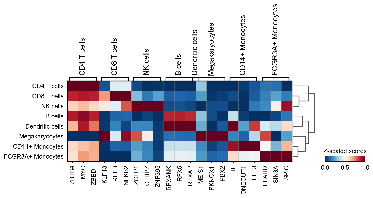
Individual TFs can be examined by plotting their score distributions.

sc.pl.violin(score, keys=["EBF1"], groupby="celltype", rotation=90)

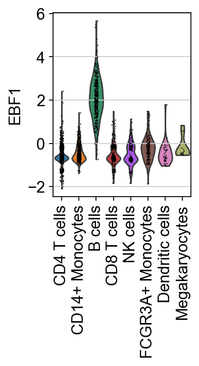
Here we can observe the TF activities for EBF1, which is a known marker TF for B cells.

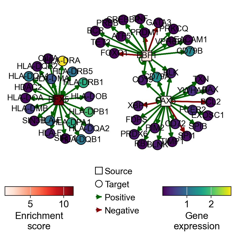
We can also plot collectri to see relevant TFs and target genes for B cells:

gex_bcells = adata[adata.obs["celltype"] == "B cells"].to_df().mean(0).to_frame().T
score_bcells = score[score.obs["celltype"] == "B cells"].to_df().mean(0).to_frame().T

dc.pl.network(
    data=gex_bcells,
    score=score_bcells,
    net=collectri,
    sources=["PAX5", "EBF1", "RFX5"],
    targets=20,
    size_node=10,
    figsize=(5, 5),
    s_cmap="Reds",
)

Pathway Scoring

The same approach used for TF scoring can also be applied to pathways. Numerous databases provide curated pathway gene sets, with one of the most well-known being MSigDB, which includes several collections [LSP+11]. These and many other resources can be accessed using the function decoupler.op.resource(). To view the list of available databases, use decoupler.op.show_resources().

PROGENy Pathway Genes

PROGENy is a comprehensive resource that provides a curated collection of pathways and their target genes, along with weights for each interaction [SKK+18].

Below is a brief description of each pathway:

• Androgen: involved in the growth and development of the male reproductive organs

• EGFR: regulates growth, survival, migration, apoptosis, proliferation, and differentiation in mammalian cells

• Estrogen: promotes the growth and development of the female reproductive organs

• Hypoxia: promotes angiogenesis and metabolic reprogramming when O2 levels are low

• JAK-STAT: involved in immunity, cell division, cell death, and tumor formation

• MAPK: integrates external signals and promotes cell growth and proliferation

• NFkB: regulates immune response, cytokine production and cell survival

• p53: regulates cell cycle, apoptosis, DNA repair and tumor suppression

• PI3K: promotes growth and proliferation

• TGFb: involved in development, homeostasis, and repair of most tissues

• TNFa: mediates haematopoiesis, immune surveillance, tumour regression and protection from infection

• Trail: induces apoptosis

• VEGF: mediates angiogenesis, vascular permeability, and cell migration

• WNT: regulates organ morphogenesis during development and tissue repair

This is how to access to it.

progeny = dc.op.progeny(organism="human")
progeny

	source	target	weight	padj
0	Androgen	TMPRSS2	11.490631	2.384806e-47
1	Androgen	NKX3-1	10.622551	2.205102e-44
2	Androgen	MBOAT2	10.472733	4.632376e-44
3	Androgen	KLK2	10.176186	1.944410e-40
4	Androgen	SARG	11.386852	2.790210e-40
...	...	...	...	...
62456	p53	ENPP2	2.771405	4.993215e-02
62457	p53	ARRDC4	3.494328	4.996747e-02
62458	p53	MYO1B	-1.148057	4.997905e-02
62459	p53	CTSC	-1.784693	4.998864e-02
62460	p53	NAA50	-1.435013	4.998884e-02

62461 rows × 4 columns

Scoring

Pathway scores can be easily computed by running the ulm method.

dc.mt.ulm(data=adata, net=progeny)

Scores can be then extracted.

score = dc.pp.get_obsm(adata=adata, key="score_ulm")
score

AnnData object with n_obs × n_vars = 2638 × 14
    obs: 'n_genes', 'percent_mito', 'n_counts', 'celltype', 'leiden'
    uns: 'draw_graph', 'louvain', 'louvain_colors', 'neighbors', 'pca', 'rank_genes_groups', 'leiden_colors', 'dendrogram_leiden', 'celltype_colors', 'dendrogram_celltype'
    obsm: 'X_pca', 'X_tsne', 'X_umap', 'X_draw_graph_fr', 'score_ulm', 'padj_ulm'

And visualized.

sc.pl.umap(score, color=["Trail", "celltype"], cmap="RdBu_r", vcenter=0)
sc.pl.violin(score, keys=["Trail"], groupby="celltype", rotation=90)

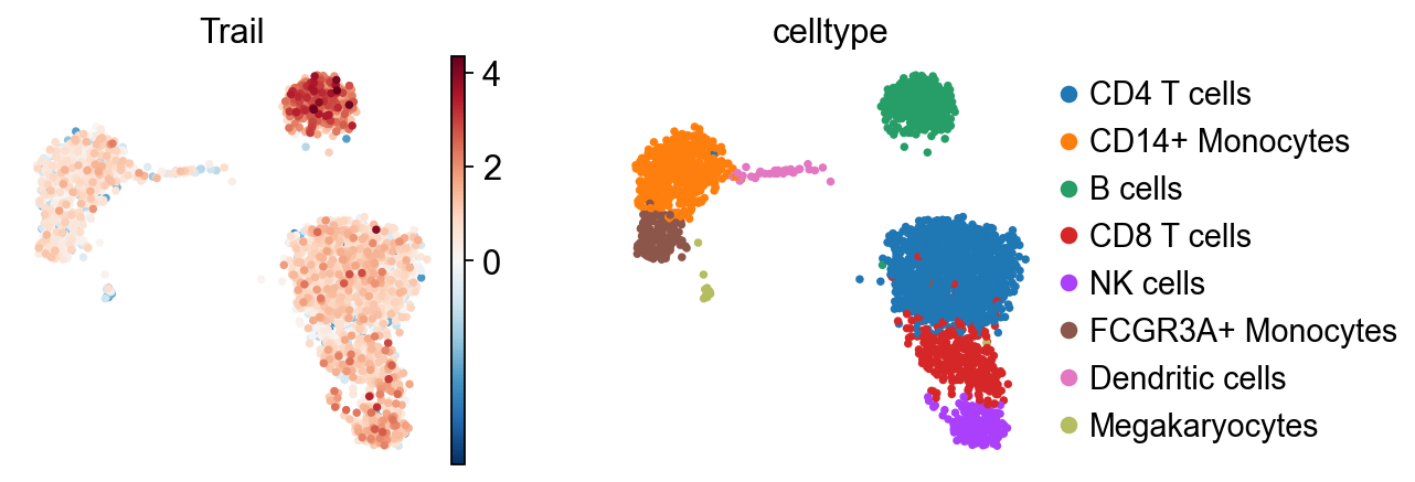
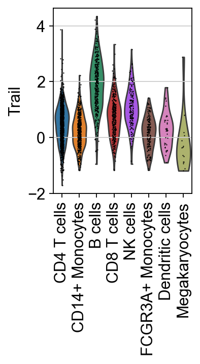
It seem that in B cells, the pathway Trail, associated with apoptosis, is more active.

Given that there are only 14 pathways, they can be directly visualized without the need for marker extraction.

sc.pl.matrixplot(
    adata=score,
    var_names=score.var_names,
    groupby="celltype",
    dendrogram=True,
    standard_scale="var",
    colorbar_title="Z-scaled scores",
    cmap="RdBu_r",
)

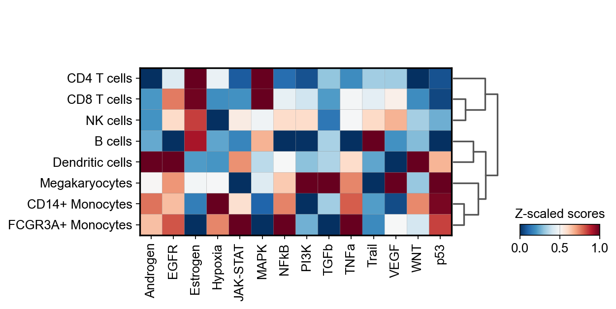
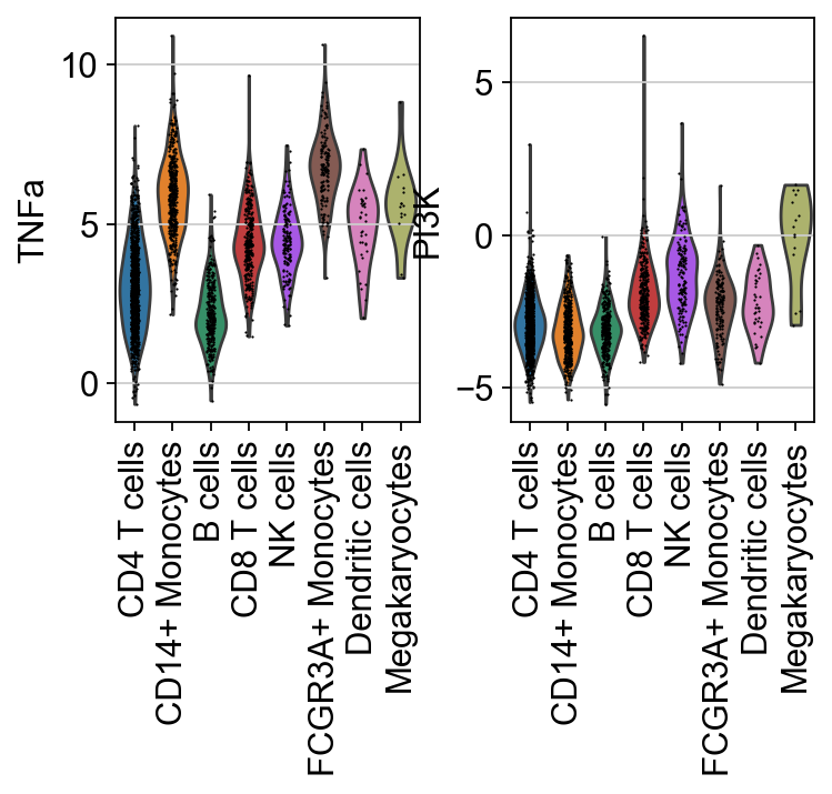
In this specific example, it can be observed that TNF-α is more active in FCGR3A+ Monocytes, while PI3K activity is higher in Megakaryocytes.

sc.pl.violin(score, keys=["TNFa", "PI3K"], groupby="celltype", rotation=90)

Hallmark gene sets

Hallmark gene sets are curated collections of genes that represent specific, well-defined biological states or processes. They are part of MSigDB and were developed to reduce redundancy and improve interpretability compared to older, more overlapping gene set collections [LSP+11].

A total of 50 gene sets are provided, designed to be non-redundant, concise, and biologically coherent.

This is how to access them.

hallmark = dc.op.hallmark(organism="human")
hallmark

	source	target
0	IL2_STAT5_SIGNALING	MAFF
1	COAGULATION	MAFF
2	HYPOXIA	MAFF
3	TNFA_SIGNALING_VIA_NFKB	MAFF
4	COMPLEMENT	MAFF
...	...	...
7313	PANCREAS_BETA_CELLS	STXBP1
7314	PANCREAS_BETA_CELLS	ELP4
7315	PANCREAS_BETA_CELLS	GCG
7316	PANCREAS_BETA_CELLS	PCSK2
7317	PANCREAS_BETA_CELLS	PAX6

7318 rows × 2 columns

Scoring

Pathway scores can be easily computed by running the ulm method.

dc.mt.ulm(data=adata, net=hallmark)

Scores can be then extracted.

score = dc.pp.get_obsm(adata=adata, key="score_ulm")
score

AnnData object with n_obs × n_vars = 2638 × 50
    obs: 'n_genes', 'percent_mito', 'n_counts', 'celltype', 'leiden'
    uns: 'draw_graph', 'louvain', 'louvain_colors', 'neighbors', 'pca', 'rank_genes_groups', 'leiden_colors', 'dendrogram_leiden', 'celltype_colors', 'dendrogram_celltype'
    obsm: 'X_pca', 'X_tsne', 'X_umap', 'X_draw_graph_fr', 'score_ulm', 'padj_ulm'

Next, marker gene sets for each cell type can be identified.

df = dc.tl.rankby_group(adata=score, groupby="celltype", reference="rest", method="t-test_overestim_var")
df = df[df["stat"] > 0]
df

	group	reference	name	stat	meanchange	pval	padj
3	CD4 T cells	rest	MYC_TARGETS_V1	21.490565	1.819335	1.590125e-92	1.987656e-91
8	CD4 T cells	rest	MYC_TARGETS_V2	17.441147	0.553157	4.855032e-64	2.697240e-63
11	CD4 T cells	rest	WNT_BETA_CATENIN_SIGNALING	16.358834	0.366900	6.704730e-57	2.793637e-56
22	CD4 T cells	rest	P53_PATHWAY	11.461240	0.493784	1.378643e-29	2.997051e-29
24	CD4 T cells	rest	E2F_TARGETS	9.503262	0.319374	5.152361e-21	1.030472e-20
...	...	...	...	...	...	...	...
391	Megakaryocytes	rest	IL2_STAT5_SIGNALING	0.436819	0.194693	6.665103e-01	7.934646e-01
392	Megakaryocytes	rest	PI3K_AKT_MTOR_SIGNALING	0.383430	0.163172	7.043131e-01	8.189688e-01
394	Megakaryocytes	rest	INFLAMMATORY_RESPONSE	0.105198	0.044449	9.169803e-01	9.828205e-01
395	Megakaryocytes	rest	WNT_BETA_CATENIN_SIGNALING	0.085780	0.013781	9.324955e-01	9.828205e-01
397	Megakaryocytes	rest	GLYCOLYSIS	0.071561	0.027577	9.435076e-01	9.828205e-01

218 rows × 7 columns

The top 3 set markers per cell type can then be extracted.

n_markers = 3
source_markers = (
    df.groupby("group")
    .head(n_markers)
    .drop_duplicates("name")
    .groupby("group")["name"]
    .apply(lambda x: list(x))
    .to_dict()
)
source_markers

{'B cells': ['KRAS_SIGNALING_DN',
  'ALLOGRAFT_REJECTION',
  'INTERFERON_GAMMA_RESPONSE'],
 'CD14+ Monocytes': ['COMPLEMENT',
  'ANGIOGENESIS',
  'EPITHELIAL_MESENCHYMAL_TRANSITION'],
 'CD4 T cells': ['MYC_TARGETS_V1',
  'MYC_TARGETS_V2',
  'WNT_BETA_CATENIN_SIGNALING'],
 'CD8 T cells': ['ANDROGEN_RESPONSE', 'APICAL_JUNCTION'],
 'Dendritic cells': ['OXIDATIVE_PHOSPHORYLATION',
  'FATTY_ACID_METABOLISM',
  'ADIPOGENESIS'],
 'FCGR3A+ Monocytes': ['COAGULATION'],
 'Megakaryocytes': [],
 'NK cells': ['INTERFERON_ALPHA_RESPONSE']}

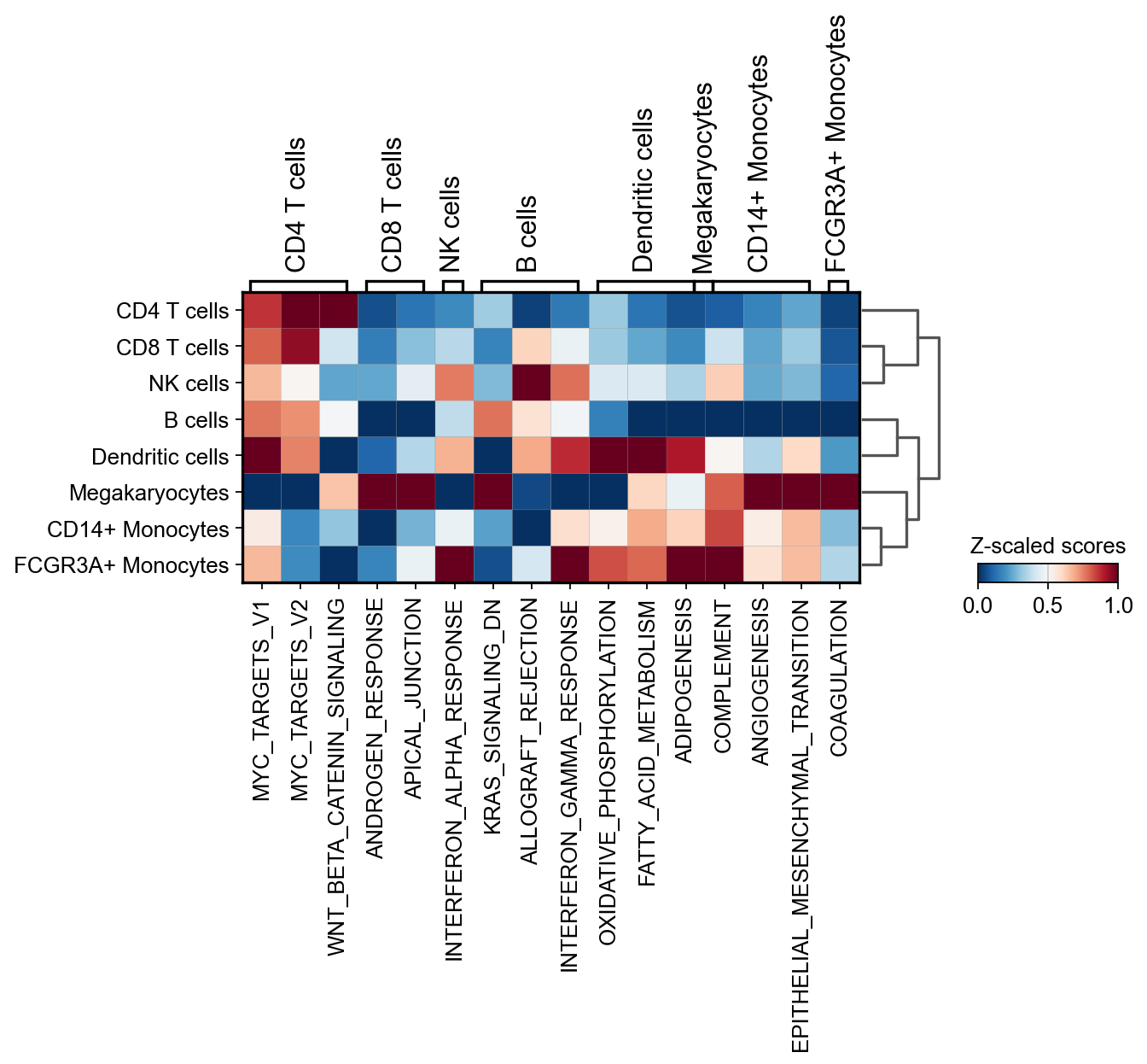
And plotted.

sc.pl.matrixplot(
    adata=score,
    var_names=source_markers,
    groupby="celltype",
    dendrogram=True,
    standard_scale="var",
    colorbar_title="Z-scaled scores",
    cmap="RdBu_r",
)