Benchmarking pipeline

Enrichment analysis involves combining a statistical enrichment method with a prior knowledge network that defines sets of features. A key question is whether the choice of enrichment method or the prior network influences the performance of the resulting scores. When perturbation experiments are available, enrichment methods and prior networks can be benchmarked by evaluating their ability to recover known perturbed regulators.

This notebook demonstrates the use of decoupler for benchmarking enrichment methods and prior knowledge networks using transcription factor (TF) perturbation experiments.

In the first part of this vignette, a toy dataset is employed to benchmark enrichment methods using a fixed prior knowledge network. In the second part, single-gene perturbation data from the KnockTF2 database, a literature-curated resource of perturbation experiments [FSL+19], is used to evaluate various prior knowledge networks.

Evaluation metrics

To evaluate the enrichment scores obtained from a given network-method combination, their ability to distinguish perturbed from non-perturbed TFs is assessed based on the given ground truth. For instance, TFs identified in the ground truth as positively perturbed (e.g., overexpressed, phosphorylated) are expected to exhibit positive enrichment scores, whereas negatively perturbed TFs (e.g., knockdown, knockout) should display negative enrichment scores. This classification performance can be quantified using three complementary metrics.

Area Under the Curve

The Area Under the Curve (auc) metric includes both the Area Under the Receiver Operating Characteristic Curve (AUROC) and the Area Under the Precision-Recall Curve (AUPRC). Each curve is generated by applying varying significance thresholds to the enrichment scores, and the corresponding area under each curve is computed. Since AUPRC values are sensitive to class imbalance, which may vary across networks due to differences in TF coverage, a modified version of AUPRC is used, in which the performance of a random classifier is set to 0.5 [SFHG+20]. Similarly, the expected AUROC for a random classifier is also 0.5.

A summary auc score can be calculated as the harmonic mean of the AUROC and AUPRC values.

Precision and Recall (F-Score)

This score first classifies TFs into the following categories:

• True Positive (TP): TF is perturbed, and TF has significant enrichment score in the appropiate direction (+ or -)

• False Positive (FP): TF is not perturbed, but TF has significant enrichment score in any direction

• False Negative (FN): TF is perturbed, but TF does not have significant enrichment score in the appropiate direction (+ or -)

Precision and recall are then calculated as follows:

$Precision = TP / (TP + FP)$

$Recall = TP / (TP + FN)$

A summary score is computed as the harmonic mean between the precision and recall values, which is traditionally referred to as the F-score (fscore).

Quantile Normalized Ranks

This score is computed by first ranking the enrichment scores, applying quantile normalization, and then reversing the values by subtracting them from 1. As a result, the transformed scores range from 0 to 1, with higher-magnitude enrichment scores assigned values closer to 1, and lower-magnitude scores closer to 0.

The transformed scores are then grouped into two categories: TFs that belong to the ground truth (perturbed) and those that do not (non-perturbed). A one-sided p-value is calculated using the Wilcoxon rank-sum test to assess whether perturbed TFs tend to have higher quantile-normalized ranks than non-perturbed TFs. The output includes both the mean reverse-quantile-normalized rank of the perturbed TFs and the p-value from the statistical test.

A summary qrank score is then calculated as the harmonic mean of the mean reverse-quantile-normalized rank and the −log10(p-value).

Loading Packages

import numpy as np

import decoupler as dc

Evaluation of methods

Loading the dataset

adata, net = dc.ds.toy_bench()
adata

AnnData object with n_obs × n_vars = 30 × 20
    obs: 'group', 'sample', 'source', 'class', 'type_p'

The obtained anndata.AnnData consist of log-normalized gene expression values for 20 genes across 30 observations.

We can inspect the cell metadata stored in anndata.AnnData.obs.

adata.obs.head(20)

	group	sample	source	class	type_p
C01	A	S01	[T1, T2]	CA	1.0
C02	A	S02	[T1, T2]	CB	1.0
C03	A	S01	[T1, T2]	CA	1.0
C04	A	S03	[T1, T2]	CB	1.0
C05	A	S02	[T1, T2]	CA	1.0
C06	A	S01	[T1, T2]	CB	1.0
C07	A	S01	[T1, T2]	CA	1.0
C08	A	S02	[T1, T2]	CB	1.0
C09	A	S02	[T1, T2]	CA	1.0
C10	A	S03	[T1, T2]	CB	1.0
C11	A	S01	[T1, T2]	CA	1.0
C12	A	S03	[T1, T2]	CB	1.0
C13	A	S02	[T1, T2]	CA	1.0
C14	A	S03	[T1, T2]	CB	1.0
C15	A	S01	[T1, T2]	CA	1.0
C16	B	S01	[T3, T4]	CB	1.0
C17	B	S01	[T3, T4]	CA	1.0
C18	B	S02	[T3, T4]	CB	1.0
C19	B	S03	[T3, T4]	CA	1.0
C20	B	S01	[T3, T4]	CB	1.0

The source column contains the ground truth for each observation, while the type_p column indicates the type of perturbation.

In this dataset, group A is expected to exhibit high positive enrichment scores for transcription factors T1 and T2, whereas group B is expected to do so for T3 and T4.

Evaluation

To evaluate method performance, enrichment scores are inferred for each method and compared to the ground truth to compute the three distinct metrics.

In this case, a random baseline method is included to illustrate how a purely random approach compares to the other methods. This is implemented using the waggr method, which supports custom functions for computing enrichment scores. This functionality also facilitates the testing of new enrichment methods without requiring full implementation from scratch.

It is also possible to specify that a consensus score should be computed based on the results across methods.

def random(x, w):
    """Random baseline method"""
    return np.random.rand(1)[0]


df = dc.bm.benchmark(
    adata=adata,
    net=net,
    kws_decouple={"cons": True, "tmin": 3, "args": {"waggr": {"fun": random}}},
)

df

	method	metric	score
0	ora	auroc	0.665370
1	ora	auprc	0.601464
2	ora	precision	0.400000
3	ora	recall	1.000000
4	ora	1-qrank	0.711667
...	...	...	...
67	consensus	auprc	0.931623
68	consensus	precision	0.000000
69	consensus	recall	0.000000
70	consensus	1-qrank	0.863333
71	consensus	-log10(pval)	19.312727

72 rows × 3 columns

Results across the different metrics can then be visualized. Here is the plot for the auc metric.

dc.bm.pl.auc(df, hue="method")

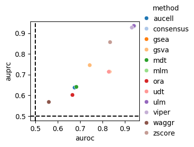
The auc metric includes both the Area Under the Receiver Operating Characteristic Curve (AUROC) and the Area Under the Precision-Recall Curve (AUPRC). Points positioned in the top right of the plot correspond to better performance scores, while those near the dashed lines indicate lower performance. The dashed lines represent the expected performance of a random classifier. As expected, the random method waggr performs the worst.

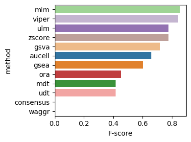
Now, here is the plot for the fscore metric.

dc.bm.pl.fscore(df, hue="method")

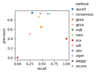
The fscore metric includes precision and recall, calculated after filtering for significant enrichment scores. As with the auc metric, points located in the top right of the plot indicate better overall performance. In this case, certain methods, such as aucell, exhibit high precision but low recall, while others show the opposite trend, such as ora. Methods such as ulm and mlm achieve a balanced performance with reasonable values for both metrics. As expected, the waggr method, representing a random baseline, performs worse than all other methods.

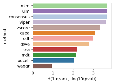
Finally, here is the plot for the qrank metric.

dc.bm.pl.qrank(df, hue="method")

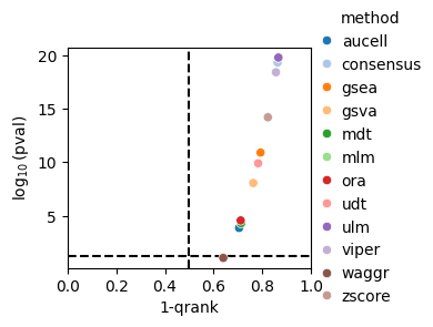
The qrank metric comprises two components, the inverse of the quantile-normalized rank of the ground truth sources (1-qrank) and the log-transformed one-sided p-value obtained from testing for differences between the ranks of sources belonging to the ground truth and those that do not (-log10(pval)). Higher values of 1-qrank and of −log10(pval) indicate better performance. Dashed lines represent the expected values for a random method, 0.5 for 1-qrank and -log10(0.05) for -log10(pval). As in previous cases, the waggr baseline behaves as a random classifier.

These pair of metrics can then be summarized using the harmonic mean between them, generating 3 aggragte metrics.

hdf = dc.bm.metric.hmean(df)
hdf

	method	auprc	auroc	H(auroc, auprc)	precision	recall	F-score	-log10(pval)	1-qrank	H(1-qrank, -log10(pval))	score
0	aucell	0.637162	0.675000	0.644387	0.947368	3.000000e-01	0.661765	3.876148	0.705000	2.040490	0.462240
1	consensus	0.931623	0.939259	0.933140	0.000000	7.733222e-17	0.000000	19.312727	0.863333	3.661881	0.777099
2	gsea	0.713912	0.830741	0.734573	0.644444	4.833333e-01	0.604167	10.908073	0.793333	3.072753	0.730810
3	gsva	0.745393	0.742407	0.744794	0.866667	4.333333e-01	0.722222	8.068603	0.763333	2.768867	0.686519
4	mdt	0.640447	0.682778	0.648488	0.500000	2.500000e-01	0.416667	4.313612	0.713333	2.146691	0.428243
5	mlm	0.935272	0.941667	0.936544	0.928571	6.500000e-01	0.855263	19.775370	0.866667	3.686995	1.000000
6	ora	0.601464	0.665370	0.613244	0.400000	1.000000e+00	0.454545	4.575803	0.711667	2.193641	0.440749
7	udt	0.713647	0.827870	0.733899	0.500000	2.500000e-01	0.416667	9.910984	0.783333	2.975857	0.658912
8	ulm	0.935204	0.939630	0.936085	0.933333	4.666667e-01	0.777778	19.775370	0.866667	3.686995	0.980342
9	viper	0.927177	0.930556	0.927851	0.925000	6.166667e-01	0.840909	18.404501	0.856667	3.611012	0.975023
10	waggr	0.567476	0.559815	0.565927	0.000000	0.000000e+00	0.000000	1.077624	0.640000	0.947981	0.000000
11	zscore	0.856637	0.833333	0.851873	0.933333	4.666667e-01	0.777778	14.204125	0.823333	3.341837	0.872048

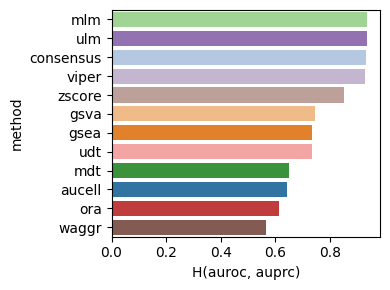
And these can also be visualized.

dc.bm.pl.bar(df=hdf, x="H(auroc, auprc)", y="method", hue="method")
dc.bm.pl.bar(df=hdf, x="F-score", y="method", hue="method")
dc.bm.pl.bar(df=hdf, x="H(1-qrank, -log10(pval))", y="method", hue="method")

Finally, the individual summary metrics can be aggregated into a single overall score, calculated as the quantile-normalized rank of their mean.

dc.bm.pl.summary(df=hdf, y="method", figsize=(6, 3))

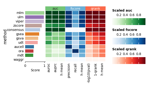
In summary, enrichment methods based on simple linear models, mlm and ulm, outperform other approaches in distinguishing perturbed from unperturbed TFs.

These findings are consistent with those reported in the original publication of decoupler, which used real TF perturbation data during evaluation [BiMVSB+22].

Evaluation of Networks

Loading the Dataset

adata = dc.ds.knocktf()
adata

AnnData object with n_obs × n_vars = 388 × 21985
    obs: 'source', 'Species', 'Knock.Method', 'Biosample.Name', 'Profile.ID', 'Platform', 'TF.Class', 'TF.Superclass', 'Tissue.Type', 'Biosample.Type', 'Data.Source', 'Pubmed.ID', 'logFC', 'type_p'

The obtained anndata.AnnData consist of log2 fold changes for ~22k genes across ~1k experiments.

We can inspect the cell metadata stored in anndata.AnnData.obs.

adata.obs

	source	Species	Knock.Method	Biosample.Name	Profile.ID	Platform	TF.Class	TF.Superclass	Tissue.Type	Biosample.Type	Data.Source	Pubmed.ID	logFC	type_p
DataSet_01_006	PROX1	Homo sapiens	siRNA	Primary lymphatic endothelial cells	GSE12846	GPL570	Homeo domain factors	Helix-turn-helix domains	Foreskin	Primary cell	GEO	18815287	-1.139770	-1
DataSet_01_007	NR2F2	Homo sapiens	siRNA	Primary lymphatic endothelial cells	GSE12846	GPL570	Nuclear receptors with C4 zinc fingers	Zinc-coordinating DNA-binding domains	Foreskin	Primary cell	GEO	18815287	-1.346960	-1
DataSet_01_008	WT1	Homo sapiens	siRNA	PLC/PRF/5	GSE12886	GPL570	C2H2 zinc finger factors	Zinc-coordinating DNA-binding domains	Liver	Cell line	GEO	19190340	-1.114740	-1
DataSet_01_010	TP53	Homo sapiens	shRNA	iPS cells	GSE13334	GPL4133	p53 domain factors	Immunoglobulin fold	Dermal_fibroblasts	Induced pluripotent stem cell	GEO	19668191	-3.137450	-1
DataSet_01_011	TP53	Homo sapiens	siRNA	U251	GSE13991	GPL1426	p53 domain factors	Immunoglobulin fold	Central_nervous_system	Cell line	GEO	19139068	-2.438950	-1
...	...	...	...	...	...	...	...	...	...	...	...	...	...	...
DataSet_04_032	FUBP1	Homo sapiens	shRNA	HepG2	ENCSR736TAW	-	Others	ENCODE_TF	Liver	Cell line	ENCODE	22955616	-1.270010	-1
DataSet_04_036	SMAD2	Homo sapiens	CRISPR	HepG2	ENCSR036ANR	-	SMAD/NF-1 DNA-binding domain factors	beta-Hairpin exposed by an alpha/beta-scaffold	Liver	Cell line	ENCODE	22955616	-1.559244	-1
DataSet_04_037	SMAD4	Homo sapiens	CRISPR	HepG2	ENCSR700FWD	-	SMAD/NF-1 DNA-binding domain factors	beta-Hairpin exposed by an alpha/beta-scaffold	Liver	Cell line	ENCODE	22955616	-1.404555	-1
DataSet_04_039	SRPK2	Homo sapiens	CRISPR	HepG2	ENCSR929EIP	-	Others	ENCODE_TF	Liver	Cell line	ENCODE	22955616	-1.392551	-1
DataSet_04_041	YBX1	Homo sapiens	CRISPR	HepG2	ENCSR548OTL	-	Cold-shock domain factors	beta-Barrel DNA-binding domains	Liver	Cell line	ENCODE	22955616	-2.025170	-1

388 rows × 14 columns

Loading the Network

For this example, we will load two prior knowledge gene regulatory networks, CollecTRI [MullerDTV+23] and DoRoThEA [GAHI+19] .

ct = dc.op.collectri()
do = dc.op.dorothea()

ct.head()

	source	target	weight	resources	references	sign_decision
0	MYC	TERT	1.0	DoRothEA-A;ExTRI;HTRI;NTNU.Curated;Pavlidis202...	10022128;10491298;10606235;10637317;10723141;1...	PMID
1	SPI1	BGLAP	1.0	ExTRI	10022617	default activation
2	SMAD3	JUN	1.0	ExTRI;NTNU.Curated;TFactS;TRRUST	10022869;12374795	PMID
3	SMAD4	JUN	1.0	ExTRI;NTNU.Curated;TFactS;TRRUST	10022869;12374795	PMID
4	STAT5A	IL2	1.0	ExTRI	10022878;11435608;17182565;17911616;22854263;2...	default activation

do.head()

	source	target	weight	confidence
0	MYC	TERT	1.0	A
1	FOS	NTS	1.0	A
2	FOS	NTF3	1.0	A
3	FOS	NFKB1	-1.0	A
4	FOS	NEFL	1.0	A

Evaluation

In this case, two analogous random networks will be generated to serve as random baselines.

rct = dc.pp.shuffle_net(ct)
rdo = dc.pp.shuffle_net(do)

And also each original network but ignoring their mode of regulation (weight) information.

unw_ct = ct.drop(columns="weight")
unw_do = do.drop(columns="weight")

To supply multiple networks to the benchmarking function, they must first be organized into a dictionary of networks. Additionally, only the ulm method is used in this case to reduce computational time.

df = dc.bm.benchmark(
    adata=adata,
    net={
        "collectri": ct,
        "dorothea": do,
        "unw_collectri": unw_ct,
        "unw_dorothea": unw_do,
        "r_collectri": rct,
        "r_dorothea": rdo,
    },
    kws_decouple={
        "methods": "ulm",
    },
)

df.head(20)

	net	metric	score
0	collectri	auroc	0.719133
1	collectri	auprc	0.760249
2	collectri	precision	0.007339
3	collectri	recall	0.315412
4	collectri	1-qrank	0.728525
5	collectri	-log10(pval)	39.321597
0	dorothea	auroc	0.687706
1	dorothea	auprc	0.721169
2	dorothea	precision	0.010575
3	dorothea	recall	0.359813
4	dorothea	1-qrank	0.692722
5	dorothea	-log10(pval)	21.809839
0	unw_collectri	auroc	0.658961
1	unw_collectri	auprc	0.705306
2	unw_collectri	precision	0.005095
3	unw_collectri	recall	0.286738
4	unw_collectri	1-qrank	0.674280
5	unw_collectri	-log10(pval)	23.350754
0	unw_dorothea	auroc	0.626609
1	unw_dorothea	auprc	0.678251

Results across the different metrics can then be visualized. Here is the plot for the auc metric.

dc.bm.pl.auc(df, hue="net")

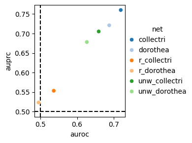
Similarly, here is the plot for the fscore metric.

dc.bm.pl.fscore(df, hue="net")

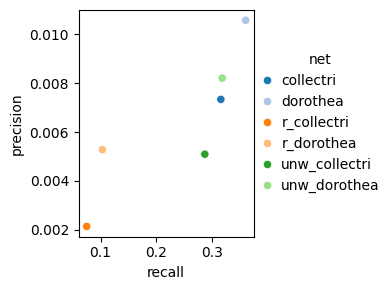
And for the qrank metric.

dc.bm.pl.qrank(df, hue="net")

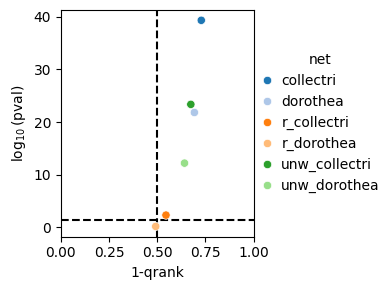
As expected, the random networks are unable to distinguish between perturbed and unperturbed TFs based on the obtained enrichment scores.

Next, the summary statistics can be generated.

hdf = dc.bm.metric.hmean(df)
hdf

	net	auprc	auroc	H(auroc, auprc)	precision	recall	F-score	-log10(pval)	1-qrank	H(1-qrank, -log10(pval))	score
0	collectri	0.760249	0.719133	0.751654	0.007339	0.315412	0.009120	39.321597	0.728525	3.391298	1.000000
1	dorothea	0.721169	0.687706	0.714218	0.010575	0.359813	0.013123	21.809839	0.692722	3.073169	0.897834
2	r_collectri	0.553499	0.536420	0.549997	0.002139	0.075269	0.002655	2.311545	0.545284	1.402780	0.361641
3	r_dorothea	0.523412	0.495025	0.517477	0.005282	0.103286	0.006519	0.161909	0.491971	0.187001	0.000000
4	unw_collectri	0.705306	0.658961	0.695523	0.005095	0.286738	0.006340	23.350754	0.674280	3.022308	0.875649
5	unw_dorothea	0.678251	0.626609	0.667253	0.008210	0.317757	0.010196	12.184879	0.641430	2.649298	0.760155

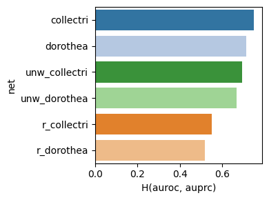
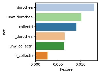
And visualized.

dc.bm.pl.bar(df=hdf, x="H(auroc, auprc)", y="net", hue="net")
dc.bm.pl.bar(df=hdf, x="F-score", y="net", hue="net")
dc.bm.pl.bar(df=hdf, x="H(1-qrank, -log10(pval))", y="net", hue="net")

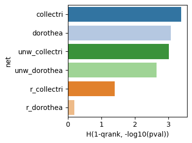
Finally, the individual summary metrics can be aggregated into a single overall score, calculated as the quantile-normalized rank of their mean.

dc.bm.pl.summary(df=hdf, y="net", figsize=(7, 3))

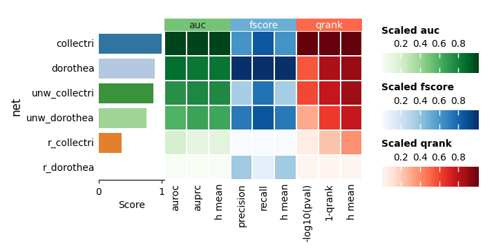
As expected, either removing the mode of regulation (weight) or shuffling target genes leads to a decrease in evaluation performance.