decoupler.mt.ora#

decoupler.mt.ora = <decoupler._Method.Method object>#

Over Representation Analysis (ORA) [Fis22].

This approach first creates a contingency table.

2×2 Contingency Table#
	$\in F$	$\notin F$
$\in Sign. features$	$a$	$b$
$\notin Sign. features$	$c$	$d$

Where:

$a$ is the number of features that are both significant and in $F$
$b$ is the number of features that are signficiant but not in $F$
$c$ is the number of features that are not signficiant but in $F$
$d$ is the number of features that are not signficiant and not in $F$

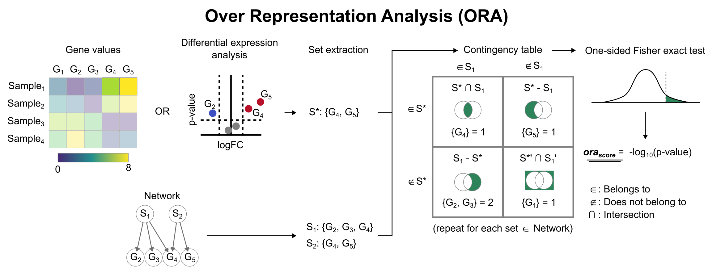
Over Representation Analysis (ORA) schematic. — Over Representation Analysis (ORA) scheme.#

The statistic is calculated as the Odds Ratio $OR$ with Haldane-Anscombe correction.

\text{OR} = \log{\frac{\frac{a + 0.5}{b + 0.5}}{\frac{c + 0.5}{d + 0.5}}}

And the $p_{value}$ is obtained afer computing a two-tailed Fisher’s exact test with the same table.

Finally, the obtained $p_{value}$ are adjusted by Benjamini-Hochberg correction.

Parameters:

data –
anndata.AnnData instance, pandas.DataFrame, or a tuple of (matrix, samples, features). All methods assume that input values follow a normal distribution unless otherwise specified. Therefore, when working with observational count data, some form of normalization is required (e.g., scanpy’s library-size normalization followed by log1p). Using raw integer counts is not recommended, as they follow a Poisson distribution.

Feature scaling on normalized counts is also acceptable, but note that it changes the results by assuming equal importance across features, and outcomes will vary depending on which observations are included.

No normalization or transformation is required when using contrast-level feature statistics such as log fold changes or Wald test statistics.
net – Dataframe in long format. Must include source and target columns, and optionally a weight column.
tmin (default: 5) – Minimum number of targets per source. Sources with fewer targets will be removed.
layer – Layer key name of an anndata.AnnData instance.
raw (default: False) – Whether to use the .raw attribute of anndata.AnnData.
empty (default: True) – Whether to remove empty observations (rows) or features (columns).
bsize (default: 250000) – For large datasets in sparse format, this parameter controls how many observations are processed at once. Increasing this value speeds up computation but uses more memory.
verbose (default: False) – Whether to display progress messages and additional execution details.
n_up – Number of top-ranked features, based on their magnitude, to select as observed features. If None, the top 5% of positive features are selected.
n_bm – Number of bottom-ranked features, based on their magnitude, to select as observed features.
n_bg – Number indicating the background size.
ha_corr – Haldane-Anscombe correction of odds ratio.

Returns:

Enrichment scores $ES$ and, if applicable, adjusted $p_{value}$ by Benjamini-Hochberg.

Example

import decoupler as dc

adata, net = dc.ds.toy()
dc.mt.ora(adata, net, tmin=3)

decoupler.mt.ora

Contents

decoupler.mt.ora#