decoupler.mt.mlm

decoupler.mt.mlm = <decoupler._Method.Method object>

Multivariate Linear Model (MLM) [BiMVSB+22].

This approach uses the molecular features from one observation as the population of samples and it fits a linear model with with multiple covariates, which are the weights of all feature sets $F$.

$$y^i = \beta_0 + \beta_1 x_{1}^{i} + \beta_2 x_{2}^{i} + \cdots + \beta_p x_{p}^{i} + \varepsilon$$

Where:

• $y^i$ is the observed feature statistic (e.g. gene expression, $log_{2}FC$, etc.) for feature $i$

• $x_{p}^{i}$ is the weight of feature $i$ in feature set $F_p$. For unweighted sets, membership in the set is indicated by 1, and non-membership by 0.

• $\beta_0$ is the intercept

• $\beta_p$ is the slope coefficient for feature set $F_p$

• $\varepsilon$ is the error term for feature $i$

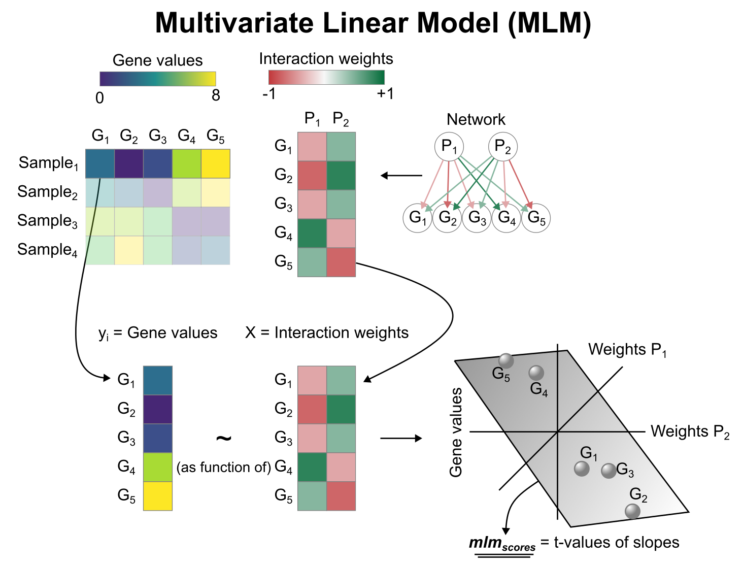
Multivariate Linear Model (MLM) scheme. In this example, the observed gene expression of $Sample_1$ is predicted using the interaction weights of two pathways, $P_1$ and $P_2$. For $P2$, since its target genes that have negative weights are lowly expressed, and its positive target genes are highly expressed, the relationship between the two variables is positive so the obtained $ES$ score is positive. Scores can be interpreted as active when positive, repressive when negative, and inconclusive when close to 0.

The enrichment score $ES$ for each $F$ is then calculated as the t-value of the slope coefficients.

$$ES = t_{\beta_1} = \frac{\hat{\beta}_1}{\mathrm{SE}(\hat{\beta}_1)}$$

Where:

• $t_{\beta_1}$ is the t-value of the slope

• $\mathrm{SE}(\hat{\beta}_1)$ is the standard error of the slope

Next, $p_{value}$ are obtained by evaluating the two-sided survival function ($sf$) of the Student’s t-distribution.

$$p_{value} = 2 \times \mathrm{sf}(|ES|, \text{df})$$

Parameters:

• data –

  anndata.AnnData instance, pandas.DataFrame, or a tuple of (matrix, samples, features). All methods assume that input values follow a normal distribution unless otherwise specified. Therefore, when working with observational count data, some form of normalization is required (e.g., scanpy’s library-size normalization followed by log1p). Using raw integer counts is not recommended, as they follow a Poisson distribution.

  Feature scaling on normalized counts is also acceptable, but note that it changes the results by assuming equal importance across features, and outcomes will vary depending on which observations are included.

  No normalization or transformation is required when using contrast-level feature statistics such as log fold changes or Wald test statistics.

• net – Dataframe in long format. Must include source and target columns, and optionally a weight column.

• tmin (default: 5) – Minimum number of targets per source. Sources with fewer targets will be removed.

• layer – Layer key name of an anndata.AnnData instance.

• raw (default: False) – Whether to use the .raw attribute of anndata.AnnData.

• empty (default: True) – Whether to remove empty observations (rows) or features (columns).

• bsize (default: 250000) – For large datasets in sparse format, this parameter controls how many observations are processed at once. Increasing this value speeds up computation but uses more memory.

• verbose (default: False) – Whether to display progress messages and additional execution details.

• tval – Whether to return the t-value (tval=True) the coefficient of the fitted model (tval=False).

Returns:

Enrichment scores $ES$ and, if applicable, adjusted $p_{value}$ by Benjamini-Hochberg.

Example

import decoupler as dc

adata, net = dc.ds.toy()
dc.mt.mlm(adata, net, tmin=3)