Usage

decoupler provides various statistical methods to infer enrichment scores from omics data using prior knowledge [BiMVSB+22].

It is a package from the scverse ecosystem [VBH+23], designed for easy interoperability with anndata and scanpy [WAT18].

Enrichment analysis tests whether a specific set of omics features is “overrepresented” or “coordinated” in the measured data compared to a background distribution. These sets are predefined based on existing biological knowledge and may vary depending on the omics technology used.

Enrichment analysis can be performed at two distinct resolutions:

1. Observation level: Feature set enrichment scores are computed individually for each observation or sample within the dataset. This is useful for characterizing continous processes that cannot be easily splitted into groups.

2. Contrast level: When the dataset includes defined groups, differential testing statistics can be derived between groups and subsequently used to compute a final vector of feature set enrichment scores.

This notebook provides a brief demonstration of inferring enrichment scores at the observation level using a toy dataset. For more detailed tutorials, refer to the other vignettes.

Note

In Jupyter Notebooks and JupyterLab, documentation for a Python function can be accessed by pressing SHIFT + TAB (twice to expand) or by typing ?<function_name>.

Loading Packages

Note

The first time decoupler is run in an environment, execution may be slow due to Numba compiling its source code. Subsequent runs are faster, as the compiled code is cached.

import scanpy as sc
import decoupler as dc

sc.set_figure_params(figsize=(3.5, 3.5), frameon=False)

Loading The Dataset

adata, net = dc.ds.toy()

The obtained anndata.AnnData consist of log-normalized integer transcript counts for 30 cells with measurements for 20 genes.

adata

AnnData object with n_obs × n_vars = 30 × 20
    obs: 'group', 'sample'

Cells are belong to two distinct groups, “A” and “B”, which exhibit differences in gene expression.

sc.pl.heatmap(
    adata=adata,
    groupby="group",
    var_names=adata.var_names,
)
sc.pl.violin(adata, groupby="group", keys=["G01", "G05", "G13"], size=5)

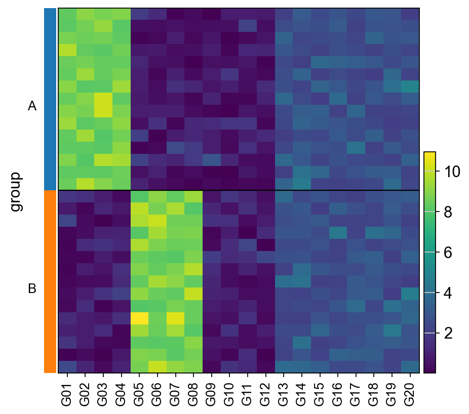
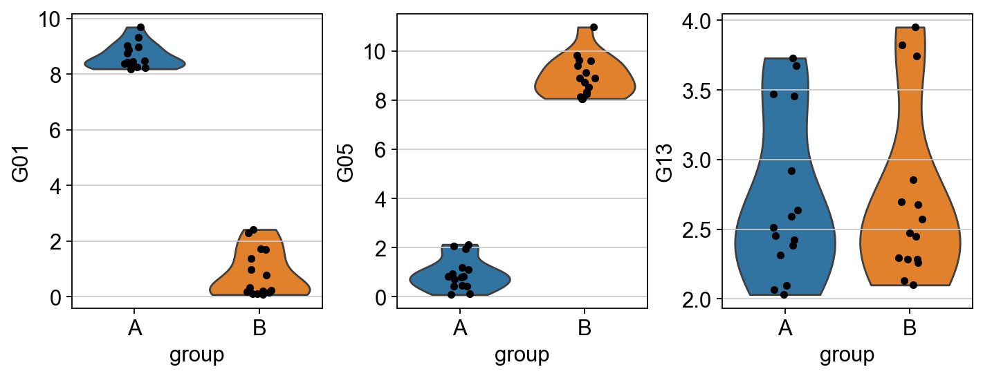
Some genes are more expressed in group A (like G01), others in group B (like G05) and others there is no difference (like G13). Ideally, these differences in gene expression programs should be captured in terms of interpretable biological entities. In this example, this is achieved by summarizing gene expression into transcription factor (TF) enrichment scores.

This toy dataset also includes a simple network comprising five TFs with defined regulatory interactions, either positive or negative, with target genes (Gs).

net

	source	target	weight
0	T1	G01	1.0
1	T1	G02	1.0
2	T1	G03	0.7
3	T2	G04	1.0
4	T2	G06	-0.5
5	T2	G07	-3.0
6	T2	G08	-1.0
7	T3	G06	1.0
8	T3	G07	0.5
9	T3	G08	1.0
10	T4	G05	1.9
11	T4	G10	-1.5
12	T4	G11	-2.0
13	T4	G09	3.1
14	T5	G09	0.7
15	T5	G10	1.1
16	T5	G11	0.1

This network can also be visualized like a graph.

dc.pl.network(net, size_node=15, s_cmap="white", t_cmap="white", c_pos_w="darkgreen", c_neg_w="darkred", figsize=(5, 5))

Based on this network, and the observed pattern of gene expression, cells in group “A” are expected to exhibit positive activity for T1 and T2, while cells in group “B” should show high activity for T3 and T4. T5 is not expected to display activity in any of the cells.

Enrichment Methods

decoupler contains multiple enrichment methods.

dc.mt.show()

	name	desc	stype	weight	test	limits	reference
0	aucell	AUCell	categorical	False	False	(0, 1)	https://doi.org/10.1038/nmeth.4463
1	gsea	Gene Set Enrichment Analysis (GSEA)	numerical	False	True	(-inf, inf)	https://doi.org/10.1073/pnas.0506580102
2	gsva	Gene Set Variation Analysis (GSVA)	numerical	False	False	(-1, 1)	https://doi.org/10.1186/1471-2105-14-7
3	mdt	Multivariate Decision Tree (MDT)	numerical	True	False	(0, 1)	https://doi.org/10.1093/bioadv/vbac016
4	mlm	Multivariate Linear Model (MLM)	numerical	True	True	(-inf, inf)	https://doi.org/10.1093/bioadv/vbac016
5	ora	Over Representation Analysis (ORA)	categorical	False	True	(-inf, inf)	https://doi.org/10.2307/2340521
6	udt	Univariate Decision Tree (UDT)	numerical	True	False	(0, 1)	https://doi.org/10.1093/bioadv/vbac016
7	ulm	Univariate Linear Model (ULM)	numerical	True	True	(-inf, inf)	https://doi.org/10.1093/bioadv/vbac016
8	viper	Virtual Inference of Protein-activity by Enric...	numerical	True	True	(-inf, inf)	https://doi.org/10.1038/ng.3593
9	waggr	Weighted Aggregate (WAGGR)	numerical	True	True	(-inf, inf)	https://doi.org/10.1093/bioadv/vbac016
10	zscore	Z-score (ZSCORE)	numerical	True	True	(-inf, inf)	https://doi.org/10.1038/s41467-021-21211-6

Each method infers enrichment scores using different types of statistic (categorical or numerical), some incorporate feature weights, others perform statistical testing and return p-values, and the resulting scores may vary in their numerical range.

Consequently, methods may have specific arguments, which can be viewed by running ?decoupler.mt.<method_name>.

To have a unified framework, methods inside decoupler have these shared arguments:

• data: AnnData instance, DataFrame or tuple of [matrix, samples, features]

• net: Dataframe in long format. Must include source and target columns, and optionally a weight column:

  • source: feature set names, for example: TFs, pathways, cell types, etc.

  • target: feature names, for example: genes regulated by a TF, phosphosites modified by a Kinase, etc.

  • weight: (optional): strength of the source-target interaction. Will be used by enrichment methods that model feature weights. Can be any value between -∞ and +∞

• tmin: Minimum number of targets per source. Sources with fewer targets will be removed

• raw: Whether to use the .raw attribute of anndata.AnnData

• empty: Whether to remove empty observations (rows) and features (columns)

• bsize: For large datasets in sparse format, this parameter controls how many observations are processed at once. Increasing this value speeds up computation but uses more memory

• verbose: Whether to display progress messages and additional execution details

Running Methods

Individual methods

As an example, the Gene Set Enrichment Analysis (gsea) method [LSP+11], one of the most widely used statistical approaches, will be run first.

dc.mt.gsea(data=adata, net=net, tmin=0)

The resulting enrichment scores can then be visualized.

scores = dc.pp.get_obsm(adata, key="score_gsea")
sc.pl.heatmap(
    adata=scores,
    groupby="group",
    var_names=scores.var_names,
    cmap="RdBu_r",
    vcenter=0,
)

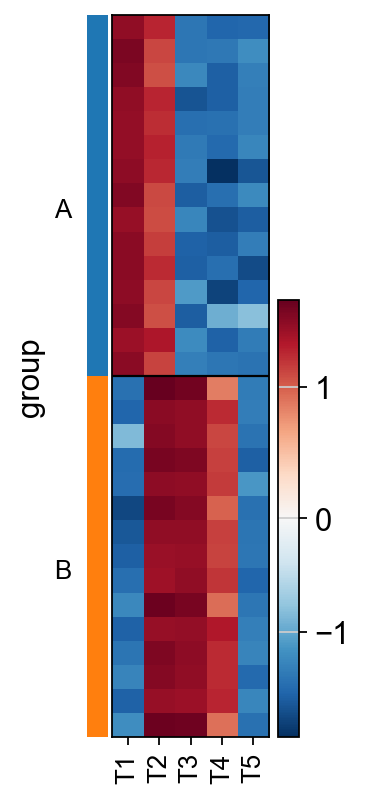
For TFs T1 and T3, the inferred activities effectively distinguish between the two groups of cells. In contrast, T2 should exhibit negative enrichment scores in the “B” group due to its role as a repressor.

The misestimation of T2’s activity arises from the limitation of GSEA, which does not account for weights when inferring enrichment scores.

When weights are also available in the prior knowledge network, it is recommended to use methods that incorporate this information to obtain more accurate estimates. One such method is the Univariate Linear Model (ULM).

dc.mt.ulm(data=adata, net=net, tmin=0)

As before, score can be plotted per cell.

scores = dc.pp.get_obsm(adata, key="score_ulm")
sc.pl.heatmap(
    adata=scores,
    groupby="group",
    var_names=scores.var_names,
    cmap="RdBu_r",
    vcenter=0,
)

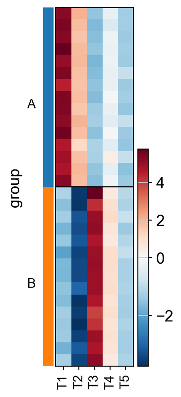
As ulm incorporates weights when estimating enrichment scores, it accurately identifies the repressor T2 as inactive in the “B” group.

Multiple Methods

decoupler enables the sequential execution of multiple methods.

For example, this line runs all available methods.

dc.mt.decouple(
    data=adata,
    net=net,
    methods="all",
    tmin=0,
)

It also can compute a consensus score based on the inferred activities across methods.

dc.mt.consensus(result=adata)

The resulting score can be visualized.

scores = dc.pp.get_obsm(adata, key="score_consensus")
sc.pl.heatmap(
    adata=scores,
    groupby="group",
    var_names=scores.var_names,
    cmap="RdBu_r",
    vcenter=0,
)

The consensus score correctly shows that T1 and T2 are active in the “A” group, while T3 and T4 are active in “B”. T5 is consistently inactive across all samples, as expected.

Access to prior knowledge

Enrichment analysis requires omics readouts and feature sets. However, feature set databases are distributed across multiple sources with varying formats and access methods, making their use more complex.

decoupler addresses this by leveraging OmniPath, a metadatabase that integrates and processes data from numerous sources [TureiKSR16]. The decoupler.op module provides a unified interface to query any database available within OmniPath.

Here is the list of available resources.

dc.op.show_resources()

	name	license
0	Adhesome	commercial
1	Almen2009	commercial
2	Baccin2019	academic
3	CORUM_Funcat	academic
4	CORUM_GO	academic
...	...	...
76	iTALK	academic
77	kinase.com	non_profit
78	scConnect	commercial
79	scConnect_complex	commercial
80	talklr	commercial

81 rows × 2 columns

As an example, SIGNOR, a database of manually curated causal relationships between human proteins and biological phenotypes, can be downloaded.

dc.op.resource("SIGNOR")

	genesymbol	pathway
0	ABL1	Cell cycle: G2/M phase transition
1	ACE	Focal segmental glomerulosclerosis
2	ACTB	Axon guidance
3	ACTN1	Axon guidance
4	ACTN1	Glutamatergic synapse
...	...	...
2943	YY1	NOTCH Signaling
2944	ZAP70	T cell activation
2945	ZAP70	P38 Signaling
2946	ZBTB16	Acute Myeloid Leukemia
2947	ZFYVE9	TGF-beta Signaling

2948 rows × 2 columns

Conclusion

Enrichment anaysis helps summarizing high-dimensional hard-to-interpret omics features into interpretable terms such as TFs or pathways.

In the original manuscript of decoupler [BiMVSB+22], we benchmarked multiple methods and found that the univariate linear model (ulm) outperformed the others. Therefore, we will use across the other vignettes.

Additionaly, decoupler provides streamlined access to a wide range of prior knowledge databases via the OmniPath metadatabase.