Cell type annotation from marker genes

In single-cell, we have no prior information of which cell type each cell belongs. To assign cell type labels, we first project all cells in a shared embedded space, then we find communities of cells that show a similar transcription profile and finally we check what cell type specific markers are expressed. If more than one marker gene is available, statistical methods can be used to test if a set of markers is enriched in a given cell population.

In this notebook we showcase how to use decoupler for cell type annotation with the 3k PBMCs 10X data-set. The data consists of 3k PBMCs from a Healthy Donor and is freely available from 10x Genomics here from this webpage

Note

This tutorial assumes that you already know the basics of decoupler. Else, check out the Usage tutorial first.

Loading packages

First, we need to load the relevant packages, scanpy to handle scRNA-seq data and decoupler to use statistical methods.

import scanpy as sc
import decoupler as dc
import numpy as np

# Plotting options, change to your liking
sc.settings.set_figure_params(dpi=200, frameon=False)
sc.set_figure_params(dpi=200)
sc.set_figure_params(figsize=(4, 4))

Single-cell processing

Loading the data-set

We can download the data easily using scanpy:

adata = sc.datasets.pbmc3k()
adata

AnnData object with n_obs × n_vars = 2700 × 32738
    var: 'gene_ids'

QC, projection and clustering

Here we follow the standard pre-processing steps as described in the scanpy vignette. These steps carry out the selection and filtration of cells based on quality control metrics and the data normalization.

Note

This is just an example, these steps should change depending on the data.

# Basic filtering
sc.pp.filter_cells(adata, min_genes=200)
sc.pp.filter_genes(adata, min_cells=3)

# Annotate the group of mitochondrial genes as 'mt'
adata.var['mt'] = adata.var_names.str.startswith('MT-')
sc.pp.calculate_qc_metrics(adata, qc_vars=['mt'], percent_top=None, log1p=False, inplace=True)

# Filter cells following standard QC criteria.
adata = adata[adata.obs.n_genes_by_counts < 2500, :].copy()
adata = adata[adata.obs.pct_counts_mt < 5, :].copy()

# Normalize the data
sc.pp.normalize_total(adata, target_sum=1e4)
sc.pp.log1p(adata)
adata.layers['log_norm'] = adata.X.copy()

Then we group cells based on the similarity of their transcription profiles. To visualize the communities we perform UMAP reduction.

# Identify the highly variable genes
sc.pp.highly_variable_genes(adata, min_mean=0.0125, max_mean=3, min_disp=0.5)

# Regress and scale the data
sc.pp.regress_out(adata, ['total_counts', 'pct_counts_mt'])
sc.pp.scale(adata, max_value=10)

# Generate PCA features
sc.tl.pca(adata, svd_solver='arpack')

# Restore X to be norm counts
dc.swap_layer(adata, 'log_norm', X_layer_key=None, inplace=True)

# Compute distances in the PCA space, and find cell neighbors
sc.pp.neighbors(adata, n_neighbors=10, n_pcs=40)

# Generate UMAP features
sc.tl.umap(adata)

# Run leiden clustering algorithm
sc.tl.leiden(adata, flavor='igraph', n_iterations=2, directed=False)

# Visualize
sc.pl.umap(adata, color='leiden', title='RNA UMAP',
           frameon=False, legend_fontweight='normal', legend_fontsize=15)

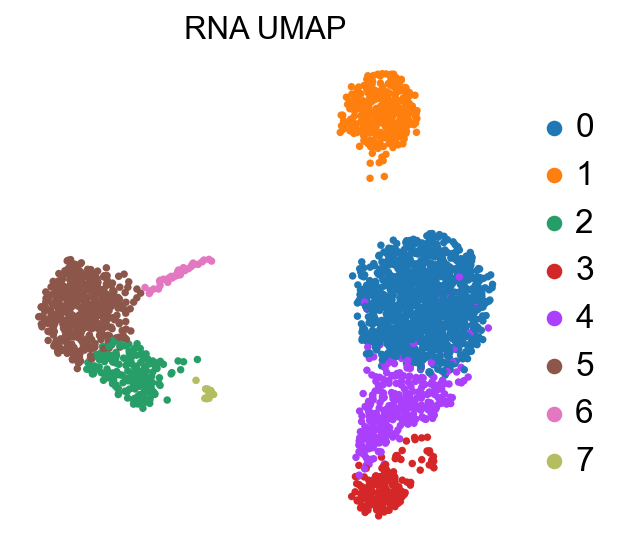
At this stage, we have identified communities of cells that show a similar transcriptomic profile, and we would like to know to which cell type they probably belong.

Marker genes

To annotate single cell clusters, we can use cell type specific marker genes. These are genes that are mainly expressed exclusively by a specific cell type, making them useful to distinguish heterogeneous groups of cells. Marker genes were discovered and annotated in previous studies and there are some resources that collect and curate them.

Omnipath is one of the largest available databases of curated prior knowledge. Among its resources, there is PanglaoDB, a database of cell type markers, which can be easily accessed using a wrapper to Omnipath from decoupler.

# Query Omnipath and get PanglaoDB
markers = dc.get_resource(
    name='PanglaoDB',
    organism='human',
    license='academic'
)
markers

	genesymbol	_entity_type	canonical_marker	cell_type	germ_layer	human	human_sensitivity	human_specificity	mouse	mouse_sensitivity	mouse_specificity	ncbi_tax_id	organ	ubiquitiousness
0	A0A068BD53	protein	True	B cells	Mesoderm	False	0.0	0.0	True	0.391473	0.00274026	10090	Immune system	0.007
1	A0A068BGV1	protein	True	Dendritic cells	Mesoderm	False	0.0	0.0	True	0.142857	0.000193013	10090	Immune system	0.0
2	A0A068BGW6	protein	True	B cells	Mesoderm	False	0.0	0.0	True	0.391473	0.00274026	10090	Immune system	0.007
3	A0A087WRN7	protein	False	Salivary mucous cells	Ectoderm	False	<NA>	<NA>	True	<NA>	<NA>	10090	Oral cavity	0.001
4	A0A0F6QAG2	protein	True	NK cells	Mesoderm	False	0.0	0.0	True	0.37234	0.000129107	10090	Immune system	0.002
...	...	...	...	...	...	...	...	...	...	...	...	...	...	...
8456	ZNF521	protein	False	Adipocyte progenitor cells	Mesoderm	True	0.0	0.0103383	False	0.0	0.0	9606	Connective tissue	0.002
8457	ZNRF4	protein	False	Germ cells	Mesoderm	True	0.28436	0.0	True	0.0	0.0	9606	Reproductive	0.01
8458	ZPBP2	protein	True	Germ cells	Mesoderm	True	0.436019	0.0	True	0.0	0.0	9606	Reproductive	0.008
8459	ZRSR2P1	protein	False	Neurons	Ectoderm	True	0.0	0.0	True	0.0	0.0	9606	Brain	0.005
8460	ZSCAN10	protein	False	Embryonic stem cells	Epiblast	True	0.0	0.000313283	True	0.0	0.0	9606	Zygote	0.0

8461 rows × 14 columns

Since our data-set is from human cells, and we want best quality of the markers, we can filter by canonical_marker and human:

# Filter by canonical_marker and human
markers = markers[markers['human'].astype(bool) & markers['canonical_marker'].astype(bool) & (markers['human_sensitivity'].astype(float) > 0.5)]

# Remove duplicated entries
markers = markers[~markers.duplicated(['cell_type', 'genesymbol'])]
markers

	genesymbol	_entity_type	canonical_marker	cell_type	germ_layer	human	human_sensitivity	human_specificity	mouse	mouse_sensitivity	mouse_specificity	ncbi_tax_id	organ	ubiquitiousness
38	AAK1	protein	False	Neurons	Ectoderm	True	0.555556	0.0320452	True	0.470588	0.0213838	9606	Brain	0.044
50	ABCA3	protein	True	Pulmonary alveolar type II cells	Endoderm	True	0.692308	0.000943693	True	0.00757576	0.000517699	9606	Lungs	0.001
85	ACADVL	protein	False	Basal cells	Mesoderm	True	0.76	0.213018	True	1.0	0.00603183	9606	Epithelium	0.05
122	ACSL5	protein	True	Enterocytes	Endoderm	True	0.666667	0.0153798	True	0.728477	0.0501211	9606	GI tract	0.055
133	ACTA2	protein	True	Smooth muscle cells	Mesoderm	True	0.904762	0.0135604	True	1.0	0.0313632	9606	Smooth muscle	0.035
...	...	...	...	...	...	...	...	...	...	...	...	...	...	...
8383	WT1	protein	False	Mesothelial cells	Mesoderm	True	1.0	0.0219436	True	0.0	0.0	9606	Epithelium	0.01
8387	XCL1	protein	False	Decidual cells	<NA>	True	1.0	0.00971482	True	0.0	0.0	9606	Reproductive	0.006
8389	XCL2	protein	False	Decidual cells	<NA>	True	1.0	0.0103416	False	0.0	0.0	9606	Reproductive	0.002
8436	ZG16	protein	False	Goblet cells	Endoderm	True	0.882353	0.00976378	True	0.0	0.0	9606	GI tract	0.013
8447	ZMYND10	protein	True	Ependymal cells	Ectoderm	True	1.0	0.0235405	True	0.0	0.0	9606	Brain	0.009

920 rows × 14 columns

For this example we will use these markers, but any collection of genes could be used. To see the list of available resources inside Omnipath, run dc.show_resources()

Enrichment with Over Representation Analysis (ORA)

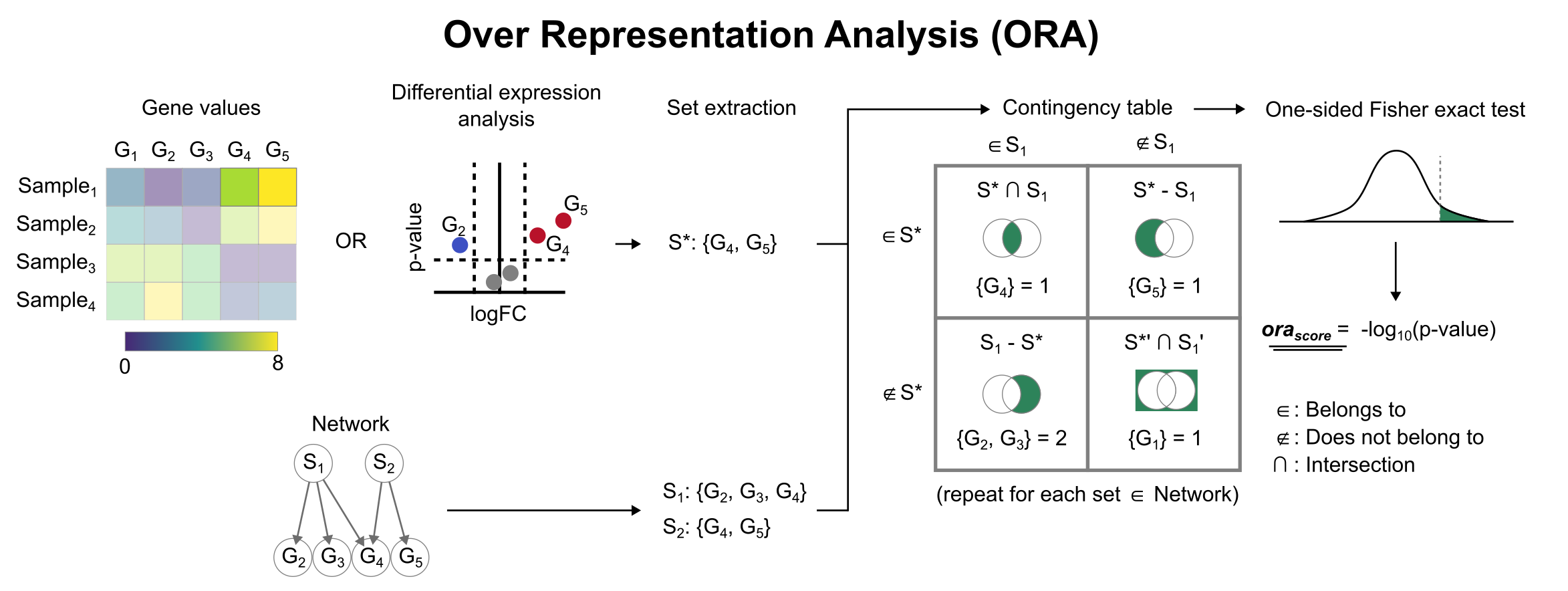
To infer functional enrichment scores we will run the Over Representation Analysis (ora) method. As input data it accepts an expression matrix (decoupler.run_ora) or the results of differential expression analysis (decoupler.get_ora_df). For the former, by default the top 5% of expressed genes by sample are selected as the set of interest (S), and for the latter a user-defined significance filtering can be used. Once we have S, it builds a contingency table using set operations for each set stored in the gene set resource being used (net). Using the contingency table, ora performs a one-sided Fisher exact test to test for significance of overlap between sets. The final score is obtained by log-transforming the obtained p-values, meaning that higher values are more significant.

We can run ora with a simple one-liner:

dc.run_ora(
    mat=adata,
    net=markers,
    source='cell_type',
    target='genesymbol',
    min_n=3,
    verbose=True,
    use_raw=False
)

1 features of mat are empty, they will be removed.
Running ora on mat with 2638 samples and 13713 targets for 49 sources.

The obtained scores (-log10(p-value))(ora_estimate) and p-values (ora_pvals) are stored in the .obsm key:

adata.obsm['ora_estimate']

source	Acinar cells	Adipocytes	Alpha cells	B cells	B cells naive	Basal cells	Decidual cells	Dendritic cells	Ductal cells	Endothelial cells	...	Plasmacytoid dendritic cells	Platelets	Podocytes	Proximal tubule cells	Pulmonary alveolar type II cells	Smooth muscle cells	T cells	T cells naive	T memory cells	Undefined placental cells
AAACATACAACCAC-1	-0.000000	1.036748	0.885021	4.739890	2.641014	0.613213	0.723628	5.546258	-0.000000	-0.000000	...	0.437907	1.871866	-0.000000	-0.0	-0.0	-0.0	11.728494	2.462920	6.821860	-0.000000
AAACATTGAGCTAC-1	-0.000000	-0.000000	0.885021	7.799678	13.894150	-0.000000	-0.000000	14.296287	0.885021	0.827013	...	1.146495	3.976687	-0.000000	-0.0	-0.0	-0.0	2.981581	1.002545	2.981581	-0.000000
AAACATTGATCAGC-1	-0.000000	0.389675	0.885021	3.427795	6.107693	-0.000000	0.723628	4.388220	-0.000000	0.298770	...	0.437907	3.976687	-0.000000	-0.0	-0.0	-0.0	11.728494	2.462920	11.728494	-0.000000
AAACCGTGCTTCCG-1	0.613213	1.036748	0.885021	2.268076	2.641014	1.542530	-0.000000	24.208278	0.885021	0.827013	...	-0.000000	8.019237	0.613213	-0.0	-0.0	-0.0	1.957728	-0.000000	1.089237	-0.000000
AAACCGTGTATGCG-1	-0.000000	-0.000000	0.885021	1.278757	0.943623	0.613213	1.793827	11.043176	-0.000000	0.298770	...	0.437907	2.858756	-0.000000	-0.0	-0.0	-0.0	1.957728	-0.000000	1.089237	1.002545
...	...	...	...	...	...	...	...	...	...	...	...	...	...	...	...	...	...	...	...	...	...
TTTCGAACTCTCAT-1	0.613213	1.036748	0.885021	3.427795	2.641014	0.613213	-0.000000	26.647907	0.885021	1.527899	...	1.146495	3.976687	-0.000000	-0.0	-0.0	-0.0	2.981581	-0.000000	-0.000000	-0.000000
TTTCTACTGAGGCA-1	-0.000000	-0.000000	0.885021	4.739890	2.641014	0.613213	-0.000000	9.543575	2.171878	0.827013	...	1.146495	3.976687	-0.000000	-0.0	-0.0	-0.0	2.981581	-0.000000	0.412702	-0.000000
TTTCTACTTCCTCG-1	-0.000000	-0.000000	0.885021	11.490976	17.770927	-0.000000	-0.000000	16.056578	-0.000000	-0.000000	...	1.146495	2.858756	-0.000000	-0.0	-0.0	-0.0	2.981581	1.002545	4.140366	-0.000000
TTTGCATGAGAGGC-1	-0.000000	-0.000000	-0.000000	4.739890	7.468516	-0.000000	-0.000000	12.626595	-0.000000	-0.000000	...	1.146495	2.858756	-0.000000	-0.0	-0.0	-0.0	2.981581	-0.000000	0.412702	1.002545
TTTGCATGCCTCAC-1	-0.000000	-0.000000	-0.000000	3.427795	4.845760	0.613213	0.723628	6.793771	0.885021	0.827013	...	1.146495	2.858756	-0.000000	-0.0	-0.0	-0.0	11.728494	2.462920	9.970169	-0.000000

2638 rows × 49 columns

Visualization

To visualize the obtained scores, we can re-use many of scanpy’s plotting functions. First though, we need to extract them from the adata object.

acts = dc.get_acts(adata, obsm_key='ora_estimate')

# We need to remove inf and set them to the maximum value observed for pvals=0
acts_v = acts.X.ravel()
max_e = np.nanmax(acts_v[np.isfinite(acts_v)])
acts.X[~np.isfinite(acts.X)] = max_e

acts

AnnData object with n_obs × n_vars = 2638 × 49
    obs: 'n_genes', 'n_genes_by_counts', 'total_counts', 'total_counts_mt', 'pct_counts_mt', 'leiden'
    uns: 'log1p', 'hvg', 'pca', 'neighbors', 'umap', 'leiden', 'leiden_colors'
    obsm: 'X_pca', 'X_umap', 'ora_estimate', 'ora_pvals'

dc.get_acts returns a new AnnData object which holds the obtained activities in its .X attribute, allowing us to re-use many scanpy functions, for example:

sc.pl.umap(acts, color=['NK cells', 'leiden'], cmap='RdBu_r')
sc.pl.violin(acts, keys=['NK cells'], groupby='leiden')

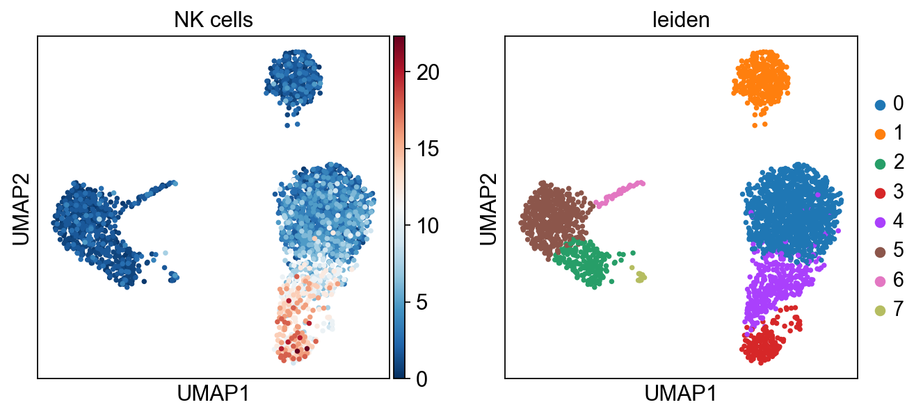
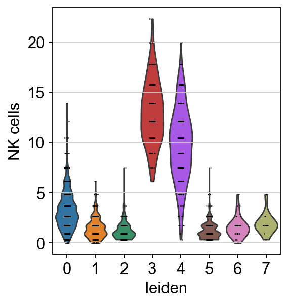
The cells highlighted seem to be enriched by NK cell marker genes.

Annotation

With decoupler we can also identify which are the top predicted cell types per cluster using the function dc.rank_sources_groups. Here, it identifies “marker” cell types per cluster using same statistical tests available in scanpy’s scanpy.tl.rank_genes_groups.

df = dc.rank_sources_groups(acts, groupby='leiden', reference='rest', method='t-test_overestim_var')
df

	group	reference	names	statistic	meanchange	pvals	pvals_adj
0	0	rest	T memory cells	41.832432	4.908299	0.000000e+00	0.000000e+00
1	0	rest	T cells	41.247917	5.483099	0.000000e+00	0.000000e+00
2	0	rest	T cells naive	32.428833	1.411612	0.000000e+00	0.000000e+00
3	0	rest	Neurons	9.510329	0.162118	4.804133e-21	1.471266e-20
4	0	rest	Decidual cells	6.015136	0.209892	2.150398e-09	4.581283e-09
...	...	...	...	...	...	...	...
387	7	rest	B cells	-3.160391	-2.461333	5.329793e-03	1.374526e-02
388	7	rest	Ductal cells	-3.456581	-0.625260	3.285145e-03	1.057917e-02
389	7	rest	T cells naive	-3.471092	-1.177413	4.621649e-03	1.258115e-02
390	7	rest	T memory cells	-3.990191	-4.116628	1.682183e-03	6.340535e-03
391	7	rest	T cells	-4.974396	-5.879572	2.552978e-04	1.389955e-03

392 rows × 7 columns

We can then extract the top 3 predicted cell types per cluster:

n_ctypes = 3
ctypes_dict = df.groupby('group').head(n_ctypes).groupby('group')['names'].apply(lambda x: list(x)).to_dict()
ctypes_dict

{'0': ['T memory cells', 'T cells', 'T cells naive'],
 '1': ['B cells naive', 'B cells', 'Langerhans cells'],
 '2': ['Macrophages', 'Dendritic cells', 'Monocytes'],
 '3': ['Gamma delta T cells', 'NK cells', 'Decidual cells'],
 '4': ['NK cells', 'Gamma delta T cells', 'Decidual cells'],
 '5': ['Neutrophils', 'Dendritic cells', 'Acinar cells'],
 '6': ['Langerhans cells', 'Dendritic cells', 'Ductal cells'],
 '7': ['Platelets', 'Endothelial cells', 'Hepatic stellate cells']}

We can visualize the obtained top predicted cell types:

sc.pl.matrixplot(acts, ctypes_dict, 'leiden', dendrogram=True, standard_scale='var',
                 colorbar_title='Z-scaled scores', cmap='RdBu_r')

WARNING: dendrogram data not found (using key=dendrogram_leiden). Running `sc.tl.dendrogram` with default parameters. For fine tuning it is recommended to run `sc.tl.dendrogram` independently.

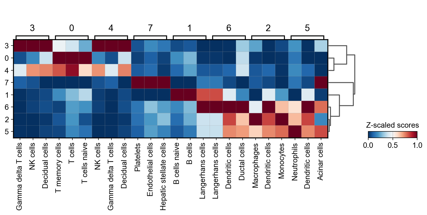
From this plot we see that cluster 7 belongs to Platelets, cluster 4 appear to be NK cells, custers 0 and 3 might be T-cells, cluster 2 should be some sort of B cells and that clusters 6,5 and 1 belong to the myeloid lineage.

We can check individual cell types by plotting their distributions:

sc.pl.violin(acts, keys=['T cells', 'B cells', 'Platelets', 'Monocytes', 'NK cells'], groupby='leiden')

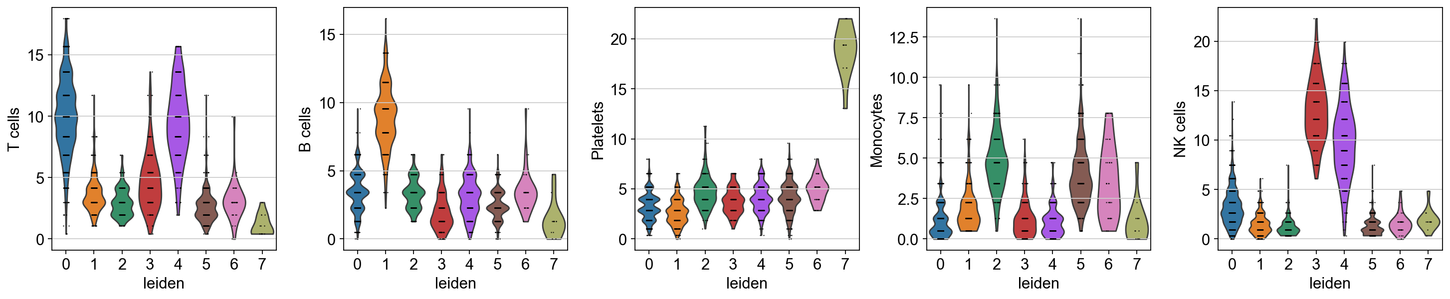
The final annotation should be done manually based on the assessment of the enrichment results. However, an automatic prediction can be made by assigning the top predicted cell type per cluster. This approach does not require expertise in the tissue being studied but can be prone to errors. Nonetheless it can be useful to generate a first draft, let’s try it:

annotation_dict = df.groupby('group').head(1).set_index('group')['names'].to_dict()
annotation_dict

{'0': 'T memory cells',
 '1': 'B cells naive',
 '2': 'Macrophages',
 '3': 'Gamma delta T cells',
 '4': 'NK cells',
 '5': 'Neutrophils',
 '6': 'Langerhans cells',
 '7': 'Platelets'}

Once we have selected the top cell type we can finally annotate:

# Add cell type column based on annotation
adata.obs['cell_type'] = [annotation_dict[clust] for clust in adata.obs['leiden']]

# Visualize
sc.pl.umap(adata, color='cell_type')

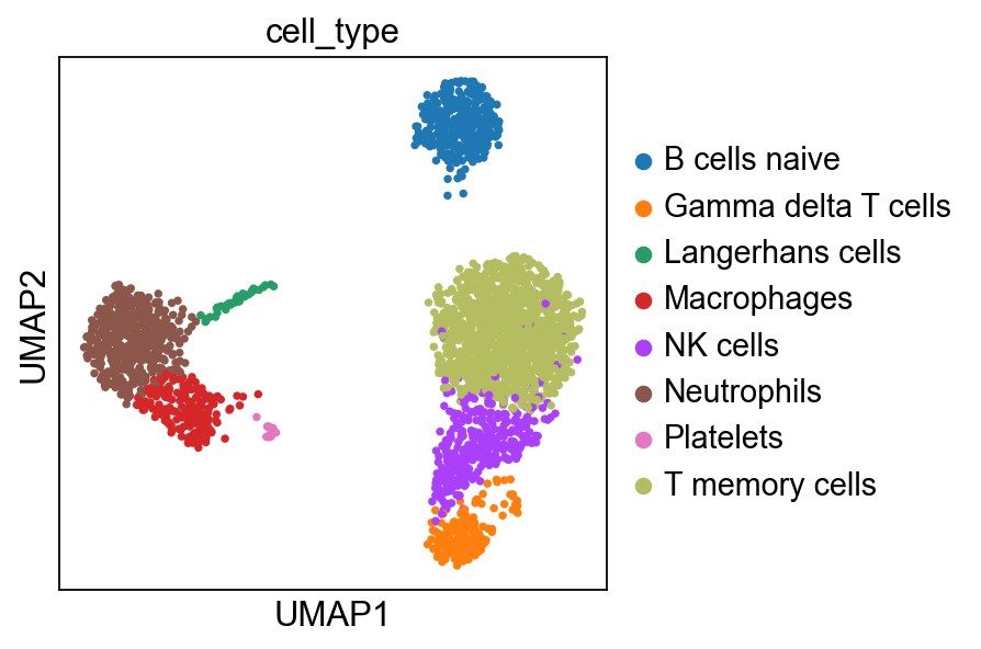
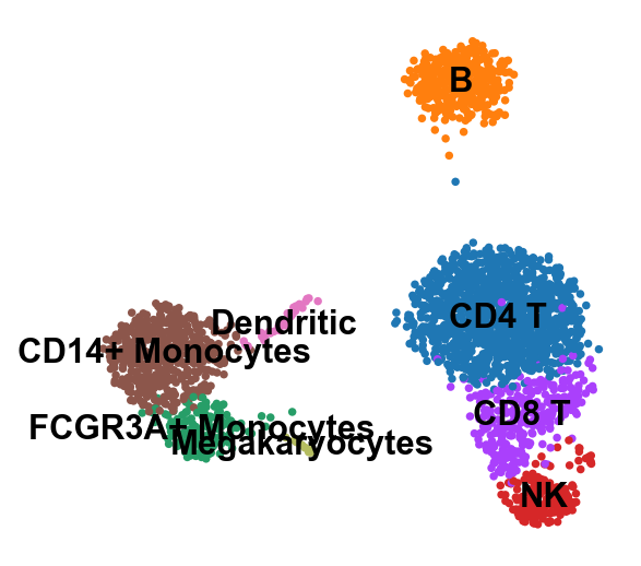
Compared to the annotation obtained by the scanpy tutorial, it is very similar but there are some errors, highlything the limitation of automatic annotation.

Note

Cell annotation should always be revised by an expert in the tissue of interest, this notebook only shows how to generate a first draft of it.